How an attention head mixes information
In the word2vec article, we learned a table of word vectors from the contexts words appeared in during training. Words with related usage could acquire related representations. But the table has a limitation: looking up a word gives the same vector regardless of the sentence it is in. Context helped train the vector; the lookup does not consult the current context.
That is the polysemy problem we left with. In “the river bank” and “the money bank,” bank retrieves the same row. Its vector can reflect evidence from both uses, but it does not tell us which use this occurrence belongs to. The surrounding words supply that missing information.
We therefore need a step after the lookup: let each position gather information from the other positions in this sentence. An attention head computes a weighted mixture of the information they carry. The weights depend on the input, so different positions can gather different mixtures. The goal is a contribution that helps make the representation useful for this particular context.
Inside a transformer block, that contribution is projected and added to the representation already there. The head computes the mixture; the residual connection incorporates the update. This gives us a path from a shared word vector to a representation enriched by its current surroundings. The next article builds the block around these updates.
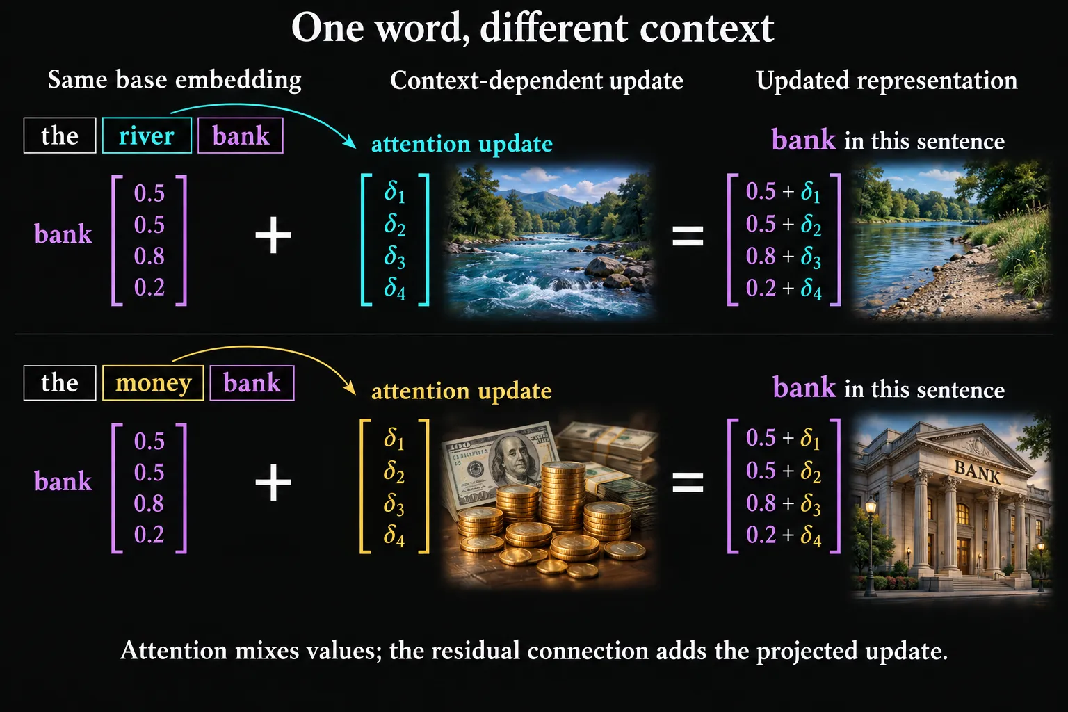
A standard transformer block contains several heads in its multi-head attention sublayer. Heads within a block run in parallel; transformer blocks run sequentially. The heads read the same input representations and compute separate mixtures, which are combined and projected into one attention update. Each subsequent block receives the previous block’s updated representations, rather than looking up the initial token vectors again.
Here we will build one head on small vectors: first watch information mix, then see how learned projections control what it gathers, and finally train a tiny model to use it.
You need vectors, dot products, and the idea that multiplying by a matrix transforms a vector. The weight-matrix article develops that last step. Our axes will be hand-chosen for legibility; real embeddings do not come with a labelled finance coordinate. We also treat each word as one token throughout this toy.
One forward pass, no training
Give four tokens four numbers each. The dimensions mean finance, water, structure, and generic content in this example only:
import numpy as np

emb = {
    #           finance water structure generic
    "the":   np.array([0.0, 0.0, 0.0, 1.0]),
    "river": np.array([0.0, 1.0, 0.0, 0.2]),
    "money": np.array([1.0, 0.0, 0.0, 0.2]),
    "bank":  np.array([0.5, 0.5, 0.8, 0.2]),
}
bank starts tied between finance and water. We want to compute a contribution at its position by mixing information from the sentence. With three tokens, the shape of that computation is:
The vectors carry information; the nonnegative weights sum to one. For now, use the embeddings themselves as those vectors. The open question is where the weights come from.
Our first rule is simple: dot the receiving token’s vector against each source vector, divide the scores by the square root of their dimension, and apply softmax. Softmax exponentiates the scores and divides each result by their sum. This makes larger scores receive larger shares while keeping the shares positive and summing to one.
Here is the reusable head. X is the sentence matrix, one token per row. We include three projection matrices now, but initially set all three to the identity, which leaves every vector unchanged.
def softmax(z):
    e = np.exp(z - z.max(axis=-1, keepdims=True))
    return e / e.sum(axis=-1, keepdims=True)

def attention(X, Wq, Wk, Wv, causal=False):
    Q, K, V = X @ Wq, X @ Wk, X @ Wv
    scores = Q @ K.T / np.sqrt(K.shape[-1])
    if causal:
        future = np.triu(np.ones(scores.shape, dtype=bool), k=1)
        scores = np.where(future, -np.inf, scores)
    A = softmax(scores)
    return A, A @ V

I = np.eye(4)
for tokens in [["the", "river", "bank"], ["the", "money", "bank"]]:
    X = np.stack([emb[t] for t in tokens])
    A, H = attention(X, I, I, I)
    print(tokens)
    print("  bank input:", X[-1])
    print("  weights:", A[-1].round(2))
    print("  mixture:", H[-1].round(2))
The result:
['the', 'river', 'bank']
  bank input: [0.5 0.5 0.8 0.2]
  weights: [0.26 0.31 0.43]
  mixture: [0.21 0.52 0.34 0.41]
['the', 'money', 'bank']
  bank input: [0.5 0.5 0.8 0.2]
  weights: [0.26 0.31 0.43]
  mixture: [0.52 0.21 0.34 0.41]
The same input vector at bank now receives different mixtures. river supplies water; money supplies finance. The mixture changes even though the weights are identical: the vectors being mixed have changed. Attention weights are only one part of the computation.
This is not yet the result of a complete transformer block. We have printed H, the head output, without an output projection or residual addition. Calling it bank’s new representation would skip those operations.
To preview the addition without introducing another matrix yet, suppose the output projection is identity and the stream has the same four coordinates. Adding the river mixture to the original gives [0.71, 1.02, 1.14, 0.61]; adding the money mixture gives [1.02, 0.71, 1.14, 0.61]. Both keep an additive contribution from the original and acquire a different context contribution. This isolates the residual operation; normalization and general output projections belong to the block article.
A plain average also separates these two sentences: the river sentence’s mean has water 0.50 and finance 0.17. So this first experiment demonstrates information mixing, not a task that requires selective attention. Our hand-designed vectors made even a simple mixture useful. Next we will see what controls that mixture and where this first matching rule falls short.
Why it mixed at all
Trace just the bank row in “the river bank.” Its unscaled dot products with the, river, and itself are [0.20, 0.54, 1.18]. Since the vectors have four dimensions, dividing by gives [0.10, 0.27, 0.59]. Softmax turns those scores into approximately [0.26, 0.31, 0.43].
Then the head computes:
mixture = 0.26 × the + 0.31 × river + 0.43 × bank
        ≈ [0.21, 0.52, 0.34, 0.41]
The displayed arithmetic is rounded; the program keeps full precision. The river term contributes water to the mixture. The largest weight happens to be on bank itself: its self-dot-product is largest in this constructed space. This is a property of these numbers, not a requirement that attention preserve identity by attending to itself. In a block, the residual path separately carries the existing representation forward.
All rows do the same operation at once. With identity projections:
scores = X @ X.T / np.sqrt(X.shape[-1])  # (n, n)
A = softmax(scores)                      # (n, n): one distribution per row
H = A @ X                               # (n, d): one mixture per row
A[i, j] is the share of source position j in the mixture received at position i. It is a distribution over positions, not over next-token vocabulary choices.
Multiply the scores by 5 before softmax: the largest score gets a larger share. Here that favors bank itself, not river. Multiply by 0.1 and the weights approach a uniform average. The standard sqrt(d_k) divisor controls score scale as query/key width changes; it does not choose which token should win. The section on dot products, cosine similarity, and scaling below explains why.
When raw similarity asks the wrong question
The first rule says “gather from vectors similar to mine.” But useful information need not resemble the receiving token. A structure can need an identity supplied by a name.
To see this cleanly, switch to a separate, two-dimensional teaching space. Its axes are structure and Paris identity. This is not a slice of the four-dimensional bank example:
# rows: the, Eiffel, tower
X2 = np.array([[0., 0.], [0., 1.], [1., 0.]])
I2 = np.eye(2)
A, H = attention(X2, I2, I2, I2)
print(A[-1].round(4))  # [0.2483 0.2483 0.5035]
print(H[-1].round(4))  # [0.5035 0.2483]
tower · Eiffel = 0. Under raw similarity, Eiffel scores exactly like the zero-vector filler. Some Paris content still enters because softmax gives both positions positive weight, but the matching rule has no way to prefer Eiffel over the filler.
For our chosen task, we want tower to gather identity information. That is a limitation of the matching rule, not a failure of weighted mixing. We need to change what tower matches against while keeping its original vector available.
Producing a query
Each token produces one query, one key, and one value vector per attention head, per transformer block. Within one head, the same learned matrix Wq transforms every position: q_i = x_i @ Wq, or Q = X @ Wq for the whole sentence. Separate projections Wk and Wv produce that token’s key and value. These are computed vectors, rather than additional vocabulary embedding lookups. A token in a block with 12 heads therefore has 12 queries, 12 keys, and 12 values. The query is a view used for matching; the original representation remains available to the rest of the block.
“What information could this position use from other tokens?” is a useful way to interpret a query. For bank, a hypothetical head might match water-related evidence or finance-related evidence; for tower, it might match a name that supplies identity. More precisely, the query determines which keys produce large dot-product scores. These scores become weights for mixing values. Producing a query is the matching setup; it has not yet gathered information or updated the token’s representation.
A query reads the token’s full current representation through Wq; it need not preserve raw similarity or keep the same number of coordinates. A large model can project thousands of representation coordinates into a much smaller query/key space. Queries and keys within a head must have the same width so their dot products are defined. Their coordinates do not have to be named concepts, and a head is not programmed with a literal question.
Transform the vector used to ask the question. A swap matrix maps tower = [1, 0] to a query [0, 1], which matches Eiffel’s identity coordinate:
swap = np.array([[0., 1.], [1., 0.]])
A, H = attention(X2, swap, I2, I2)
print(A[-1].round(4))  # [0.2483 0.5035 0.2483]
print(H[-1].round(4))  # [0.2483 0.5035]
print(X2 @ swap)
# [[0. 0.]    the's query
#  [1. 0.]    Eiffel's query
#  [0. 1.]]   tower's query
The same matrix acts on every row. Different input vectors give different queries; we did not need a separate matrix per word. The token representation and its query are now different objects: the representation supplies the input, and the query is one transformed view used for matching.
| Object | Shape | What varies? |
|---|---|---|
| Embedding table | vocabulary size × d | One learned row per token ID |
Input X | n × d | The representations in this particular sequence |
Query projection Wq | d × d_k | Shared parameters, adjusted during training |
Queries Q = X @ Wq | n × d_k | Computed for each position on this pass |
At the first layer, the input includes embeddings and any positional signal. Deeper layers operate on representations already updated by earlier layers. The projection rule is shared; its inputs need not be static word vectors.
What is query/key space, and how does it relate to subspaces?
Query/key space is the coordinate space where a head compares queries with keys. If a head uses 128 coordinates for each, both live in , and their dot product produces a matching score there. The learned maps Wq and Wk translate the much wider token representations into these matching coordinates. Each head has its own maps; the coordinates need not have named semantic meanings.
For example, a 12,288-coordinate input can be multiplied by a 12,288 × 128 query matrix to produce a 128-coordinate query. The key matrix has the same shape and produces 128-coordinate keys from the source representations. The diagram uses bank and river to show this relationship; these widths illustrate a possible model configuration, rather than the sizes of our toy.
Token representation space
12,288 dimensions in this example
The current representation carries information available to this position.
q = x @ WqEach output coordinatereads all input coordinates.
Query/key matching space
128 dimensions in this example
Wk separately maps source representations into keys with the same width.
q_bank = x_bank @ Wqk_river = x_river @ Wkscore = q_bank · k_river / √128This connects directly to row space and null space: what the matrix reads and ignores. That article uses column vectors, while our code uses row vectors. To apply its notation, set , so . Now the same subspace picture applies:
- In the 12,288-dimensional input space, the row space of contains the directions it reads. Its null space contains directions that contribute zero to the query. Adding a vector from this null space to the input leaves the query unchanged.
- In the 128-dimensional output space, the column space of contains every query the linear map can produce. It may fill all of or be a smaller subspace if the map’s rank is below 128. See column space: which outputs can the matrix reach?.
The query map can read at most 128 independent input directions in this example, leaving at least 12,160 independent input directions in its null space. Those directions are ignored by this query map; the residual stream still carries the input, and other heads or projections can use information this map ignores. The input directions read by Wq and Wk can also differ, even though their outputs are compared using the same 128 matching coordinates.
The 128-dimensional matching space is therefore a separate output space, while the relevant input subspace lies inside the original 12,288-dimensional space. In attention, “projection” usually means a learned linear map: it can stretch and mix directions and is not generally an orthogonal projection onto a plane inside the original space.
What information does the query map lose?
Make this concrete with a separate 3D → 2D example. Using the column-vector notation above, choose:
This matrix reads the two sums and . For the vector , both sums cancel:
So is in the null space. Adding any multiple of it leaves the query unchanged: . For example:
The query map cannot distinguish these two inputs. What it loses is the amount of input along the null-space direction : increasing the first two coordinates together while decreasing the third by the same amount leaves both output sums unchanged. It does not simply discard the third coordinate; that coordinate contributes to both sums. The arithmetic identifies an ignored direction; identifying any semantic information encoded along it would require experiments on a trained model.
If the keys are held fixed, these identical queries also produce identical attention scores and weights. The input change could still affect this token’s key or value, another head, or the residual stream. “Lost” here means unavailable through this query map, rather than erased from the model’s entire representation.
One query can combine several matching criteria
One query can carry several matching preferences at once. If queries and keys have 128 coordinates, their scaled dot product is:
All 128 coordinate pairs contribute to one compatibility score for this query/key pair. The query is compared with every allowed key, producing a separate score for each source position. Softmax converts those scores into one attention distribution. This is the scaled dot-product computation in the Transformer paper, §3.2.1.
128 coordinates does not mean 128 semantic features. A feature might correspond to a direction spread across many coordinates, and several features can use overlapping coordinates. Ten features could be distributed across 128 dimensions. A larger collection, such as 1,000 possible features, could in principle use overlapping directions, especially when only a few features are active at once. But 128 dimensions provide at most 128 linearly independent directions: they cannot independently preserve 1,000 arbitrary feature strengths through a linear encoding.
Toy Models of Superposition demonstrates how toy networks can represent more sparse features than dimensions, with interference between overlapping representations. This supports a representational possibility; it does not establish that a particular query contains 1,000 identifiable features or tell us what they are.
The dot product combines the evidence into one score, rather than returning a separate answer for every feature. Each head produces one attention distribution and one value mixture per receiving token. Multiple heads let different matching criteria produce separate distributions and mixtures; a single head can still combine several criteria within its own score.
Try three hypothetical matching directions
Return to the four-coordinate bank vectors, this time projecting into a three-dimensional query/key space. We hand-name its axes finance, water, and structure, and keep the key projection fixed. This is a new teaching construction, not a claim about the coordinates or behavior of a trained head.
Choose , , or to try a possible interpretation of bank’s query. Each preset changes the displayed Wq; the widget computes the resulting queries, keys, scores, and attention weights. Use to inspect the three axes, or open to combine or oppose directions.
What could this query match?
Receiving token: bank. Its input stays [0.50, 0.50, 0.80, 0.20]. Switch a hand-set Wq to change its matching direction.
1. Produce the query
q_bank = x_bank @ Wq
| Input | finance | water | structure |
|---|---|---|---|
| finance | 0.00 | 0.00 | 0.00 |
| water | 0.00 | 0.00 | 0.00 |
| structure | 0.00 | 3.75 | 0.00 |
| generic | 0.00 | 0.00 | 0.00 |
q_bank = 0.8 × [0.00, 3.75, 0.00]
= [0.00, 3.00, 0.00]
Only the structure row of this constructed Wq is nonzero. A real projection can combine every input coordinate.
Adjust Wq coefficients
Negative coefficients can make this query oppose a key direction. A zero query gives equal scores and uniform weights.
2. Compare query and keys
The query arrow is rescaled to show its direction. Scores use the full numerical query. Faded keys belong to words absent from this sentence.
3. Match first; mixing comes next
The same Wq produces a query for every token. Below, each key is computed using a fixed Wk that keeps finance, water, and structure and drops the generic coordinate.
| Token | Its query x @ Wq | Its key x @ Wk | q_bank · key / √3 | Bank's attention weight |
|---|---|---|---|---|
| the | [0.00, 0.00, 0.00] | [0.00, 0.00, 0.00] | 0.000 | 11.1% |
| river | [0.00, 0.00, 0.00] | [0.00, 1.00, 0.00] | 1.732 | 62.6% |
| bank | [0.00, 3.00, 0.00] | [0.50, 0.50, 0.80] | 0.866 | 26.3% |
The keys stay fixed when Wq changes. Switching sentences leaves bank's query unchanged here, but changes the available keys and their shares. The head would use these weights to mix values; this widget stops at matching.
These questions, axes, matrices, and token features are hand-designed teaching examples. Changing a preset changes Wq; it does not show a trained head choosing a new matrix for each sentence. Real heads learn numerical matching patterns jointly with key projections, without named semantic coordinates or literal questions.
Notice that the query need not identify a word’s intended sense on its own. In this construction, bank starts with the same input and produces the same query in both sentences. The available keys and values supply the differing context. Whether any of these hypothetical matching patterns helps a task is something training and evaluation must establish.
The embedding table and the projection matrices are separate
The embedding table E stores one starting vector per vocabulary token. The projection matrices Wq, Wk, and Wv transform a position’s current representation into its query, key, and value. Each head normally has its own projections in each transformer block; the token embedding table supplies the starting representations below the stack.
| Object | Purpose | Learned or computed? |
|---|---|---|
E | Supplies the starting vector for each token ID | Learned parameter table |
Wq, Wk, Wv | Transform the current representations | Learned projection matrices |
X, Q, K, V | Represent this input and its transformed views | Computed on each forward pass |
A, H | Weight and mix the values for this input | Computed on each forward pass |
How many tables and vectors are there?
The architecture below expands 2 heads processing 3 tokens in one standard self-attention sublayer. The embedding table is outside attention. Its selected rows become X; both heads read that same full input, using separate learned projection matrices. Within each head, Q, K, and V are computed matrices with one vector per token row. Follow the highlighted bank rows to count its queries, keys, and values across the two heads.
X · 1 input matrix · 3 × d
xthe = etheriver xriver = eriverbank xbank = ebankHead 1
3 learned projection matrices
3 computed matrices · 3 token rows each
Each token has 1 q + 1 k + 1 v in this head.
A = softmax(Q @ Kᵀ / √d_k)H(1) · 1 mixture matrix · 3 × d_vH = A @ VHead 2
3 learned projection matrices
3 computed matrices · 3 token rows each
Each token has 1 q + 1 k + 1 v in this head.
A = softmax(Q @ Kᵀ / √d_k)H(2) · 1 mixture matrix · 3 × d_vH = A @ VConcat(H(1), H(2)) · 1 matrix · 3 × (2 d_v)
One row per token, containing both head mixtures
Wo · 1 learned matrix for this sublayer · (2 d_v) × d
Δ = Concat @ Wo · 1 attention-update matrix · 3 × d
Residual addition: Y = X + Δ · the original X is added here
For n token positions and h heads in one standard self-attention sublayer:
| Object | Learned or computed? | Count | Shape of each matrix |
|---|---|---|---|
Token embedding table E | Learned | 1 for the model, before the stack | vocabulary size × d |
Input X | Computed | 1 shared input to all heads in this sublayer | n × d |
Query projections Wq | Learned | h, one per head | d × d_k |
Key projections Wk | Learned | h, one per head | d × d_k |
Value projections Wv | Learned | h, one per head | d × d_v |
Queries Q | Computed | h matrices; n h query vectors total | n × d_k |
Keys K | Computed | h matrices; n h key vectors total | n × d_k |
Values V | Computed | h matrices; n h value vectors total | n × d_v |
Query/key scores S | Computed | h, one per head | n × n |
Attention weights A | Computed | h, one per head | n × n |
Head mixtures H | Computed | h, one per head | n × d_v |
| Concatenated head outputs | Computed | 1 | n × (h d_v) |
Output projection Wo | Learned | 1 for this sublayer | (h d_v) × d |
Attention update Δ and residual result Y | Computed | 1 of each | n × d |
So one token has h queries, h keys, and h values in a block, while the block has 3h learned Q/K/V projection matrices and one output projection. A stack of N such blocks normally has its own projections in every block: 3Nh Q/K/V projection matrices and N output projections. These counts describe the standard multi-head arrangement, omit biases, and count logical matrices; implementations often pack several projections into a single parameter tensor.
Only the lookup is indexed by token ID. The projection matrices have input-coordinate rows and output-coordinate columns, so every token uses the same projection matrices within a head. Later blocks receive updated representations from the previous block, without repeating the embedding lookup. The block article adds the normalization and feed-forward details to this outline.
“Initial” describes where the lookup happens when processing a sentence. Before training from scratch, the embedding table usually starts with random numbers. Training learns those vectors jointly with the projections and the rest of the model; there is usually no separate stage that teaches the embeddings a “generic meaning” first. After training, the lookup retrieves a learned vector. It is context-independent because it does not inspect the current sentence. The same token ID retrieves the same row, even though later representations depend on context.
Our first examples use hand-set vectors so we can follow the arithmetic. The training example below learns the embedding table as well as the projections.
Three roles: matching and carrying information
The query is one of three transformed views:
| View | Computation | Job |
|---|---|---|
| Query | Q = X @ Wq | Represents what each receiving position matches against |
| Key | K = X @ Wk | Represents each source position for that matching operation |
| Value | V = X @ Wv | Supplies the vectors that will actually be mixed |
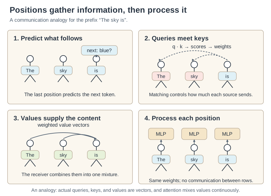
Think of token positions as people exchanging messages. Query–key matching determines the weights; values supply the messages. These are continuous vector operations. The final panel previews the per-position MLP developed in the transformer-block article.
Queries and keys meet in Q @ K.T. Both sides can be learned: the model can transform how a receiver asks and how a source is found. The two projections need not be equal, so the score from i to j can differ from the score from j to i.
Values have a different job. Keep the queries and keys fixed and swap only the value coordinates:
A, H = attention(X2, swap, I2, swap)
print(A[-1].round(4))  # [0.2483 0.5035 0.2483] -- unchanged
print(H[-1].round(4))  # [0.5035 0.2483]        -- different content
Q and K control the mixture’s weights; V controls its content. A large weight on Eiffel does not by itself tell us which direction the output moves. We must also inspect Eiffel’s value. Our swap is hand-set to make that independence visible; training will learn the transformations together.
The full head has the familiar form , as specified in the original Transformer paper, §3.2. The diagram follows its operations and dimensions, then shows the output projection used by the surrounding block:
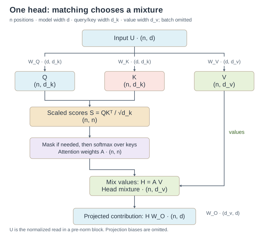
W_Q, W_K, and W_V are learned projection matrices; Q, K, and V are computed activations. In the toy example the input is X. In a pre-norm block it is a normalized read, labeled U here. The output projection maps the head mixture back to model width; residual addition comes afterward.
d_v need not equal d. A head returns a mixture in value coordinates. The block’s output projection will map it into the coordinates of the representation we are updating.
Try the two-dimensional example below. Start with , switch to , then toggle . The numbers are computed from the matrices above; changing values leaves the weights untouched.
Change the match, then change the content
The receiving position is tower. Its input is [1, 0]. Keys stay unchanged; scores use √2 scaling.
[1.0000, 0.0000][0.5035, 0.2483]Swapping the query changes the weights. Swapping values changes the mixture while leaving those weights untouched. No residual addition is shown here.
What the weight actually measures
A score compares one query/key pair. A weight compares that score with every other allowed score in the same row:
Adding another key can change a_ij without changing q_i or k_j. Likewise the weight is not a runtime word-co-occurrence count. Training changes the parameters; inference computes fresh scores and mixtures using those parameters. Position can also affect scores when positional information is supplied—we have deliberately left it out of this toy.
Dot products, cosine similarity, and scaling
We have used a dot product to compare each query with each key, then divided by . What does that division change? Compare three operations on the same vectors:
| Operation | Formula | What determines the score? |
|---|---|---|
| Dot product | Directions and vector lengths | |
| Cosine similarity | Angle only, for nonzero vectors | |
| Scaled dot product | Directions and lengths, with a fixed divisor for the head’s query/key dimension |
A dot product includes vector length
For nonzero vectors, the dot product can be written as:
It depends on both lengths and the angle between them. Take and : their dot product is . Make both vectors ten times longer, giving and , and the dot product becomes . The directions have not changed.
Hold the angle fixed in the explorer and change either length. Then hold both lengths fixed and change the angle. The vectors are labelled and here, but the same arithmetic applies to a query and a key.
Blue: vector aGreen: projectionOrange: vector b
b points right and is drawn below the line for visibility. Both vectors use the same scale.
The projection is positive: part or all of a points in the direction of b. Since b is a unit vector, the dot product equals the signed projection.
Length multiplies the signed angular contribution: making a vector longer makes a positive dot product more positive and a negative one more negative. Perpendicular vectors still give zero. A longer key therefore does not automatically receive a higher score.
Cosine similarity removes the lengths
Dividing by the product of the two lengths cancels those factors:
This is equivalent to taking the dot product after normalizing each vector to unit length. For nonzero vectors it lies between and ; it is undefined if either vector is zero.
| Query | Key | Dot product | Cosine similarity |
|---|---|---|---|
Scaling preserves the influence of lengths
In our head, is the number of coordinates in each query and key. Every pair in that head uses the same divisor , regardless of the vectors’ actual lengths.
For example, a head with divides every dot product by :
| Dot product | Scaled dot product |
|---|---|
These are illustrative scores for 64-dimensional vectors, separate from the two-dimensional examples above. Multiplying either vector by ten still multiplies its scaled dot product by ten. Dividing all scores by the same positive constant preserves their ordering and rescales their differences; it does not make the vectors unit length or bound the scores to .
Why divide by the square root of the dimension?
A dot product adds one product per coordinate:
To see how its scale can grow, assume all query and key components are independent random variables with mean zero and variance one. Each product then has mean zero and variance one:
Variances add for independent terms, so:
The expected dot product remains zero. What grows is its spread: positive and negative fluctuations become larger. At , the variance is and the standard deviation is . Dividing by brings the standard deviation back to because dividing a random variable by a constant divides its variance by the constant’s square:
This is the motivation given in the original Transformer paper, §3.2.1. It explains the choice of divisor under simplifying assumptions; learned queries and keys need not remain independent or have unit component variance, so a trained head’s score variance is not guaranteed to be one.
Scaling changes how sharply softmax chooses
Consider one query with raw scores against three keys in a four-dimensional head. Dividing by gives :
| Scores sent to softmax | Key 1 weight | Key 2 weight | Key 3 weight |
|---|---|---|---|
| Raw: | 86.7% | 11.7% | 1.6% |
| Scaled: | 66.5% | 24.5% | 9.0% |
Key 1 still wins, but receives a smaller share. Softmax responds to differences between scores: for two allowed keys, the weight ratio is . Here scaling reduces that score gap from to , changing the ratio from to . Adding the same constant to every score would leave the weights unchanged.
Large score gaps can make softmax nearly one-hot. Its derivatives with respect to its input scores then become small, which can weaken the learning signal through the attention weights. Scaling helps control this effect as query/key dimension increases. It does not prevent a trained head from learning sharp attention when useful.
Why not use cosine similarity instead?
Cosine similarity would change what the matching rule can use. Standard scaled dot-product attention retains the influence of both query/key directions and lengths. With keys fixed, increasing a query’s length by a positive factor scales its whole score row and can sharpen its attention distribution. Changing one key’s length affects that key’s score, with the effect depending on its sign.
Cosine-based attention is a possible alternative, but normalizing queries and keys removes these particular effects of their lengths. The fixed divisor instead adjusts the expected score scale as the head width changes.
Finally, keep vector normalization separate from weight normalization:
The divisor scales compatibility scores. Softmax turns each score row into nonnegative mixing weights that sum to one. Neither operation requires each query or key to have unit length.
Make it learn
Return to the bank task, but discard our hand-designed axes. The model now learns eight-dimensional embeddings and the three projection matrices. A classifier reads only the mixture at the final bank position and predicts water (0) or finance (1). It is a tiny supervised classifier, not a next-token language model or a complete transformer block.
Follow a sentence from lookup to an update
The widget uses a two-dimensional version of this classifier to keep every vector and parameter visible. Choose a sentence, then use to follow sentence → embedding lookup → Q/K/V → attention mixture → prediction → loss → gradients → parameter updates. At the gradient stage, the parameters have not changed yet. takes one SGD step; continues with the updated parameters and the other example.
Compare the embedding table with the projection matrices, then compare those stored parameters with the vectors computed from them. The gradient and update stages show all parameter groups together, including the embedding row that received no gradient because its word was absent. Use to alternate both examples, or to return to the same random initialization.
Follow one sentence through training
One head, two learned coordinates, two classes. All numbers are computed. Coordinates have no hand-assigned meaning.
Completed updates: 0. SGD learning rate: 0.3. Extra training alternates the two examples and keeps the same shared parameters.
- 1. Sentence
- 2. Lookup
- 3. Q / K / V
- 4. Mixture
- 5. Prediction
- 6. Loss
- 7. Gradients
- 8. Update
1. Sentence
Target: water. The classifier will read only the mixture at bank. The target is used by the loss, not by the attention calculation.
The parameter tables start with repeatable random numbers; the classifier bias starts at zero. Nothing has been trained separately beforehand.
This is a two-example supervised training demonstration, not a generalization test or a complete transformer block. It omits positions, normalization, residual additions, and the FFN. The Python model below uses eight coordinates and Adam; this widget uses two coordinates and SGD.
The runnable eight-dimensional model
import torch
import torch.nn as nn

vocab = {"the": 0, "river": 1, "money": 2, "bank": 3}
data = [(["the", "river", "bank"], 0),
        (["the", "money", "bank"], 1),
        (["river", "bank"], 0),
        (["money", "bank"], 1)]

def encode(tokens):
    return torch.tensor([vocab[t] for t in tokens])

class OneHeadSense(nn.Module):
    def __init__(self, vocab_size, d=8):
        super().__init__()
        self.emb = nn.Embedding(vocab_size, d)
        self.Wq, self.Wk, self.Wv = (
            nn.Linear(d, d, bias=False) for _ in range(3))
        self.cls = nn.Linear(d, 2)
        self.d = d

    def forward(self, ids, return_attn=False):
        X = self.emb(ids)
        Q, K, V = self.Wq(X), self.Wk(X), self.Wv(X)
        A = torch.softmax(Q @ K.T / self.d**0.5, dim=-1)
        H = A @ V
        logits = self.cls(H[-1])
        return (logits, A) if return_attn else logits

torch.manual_seed(0)
model = OneHeadSense(len(vocab))
opt = torch.optim.Adam(model.parameters(), lr=0.05)
loss_fn = nn.CrossEntropyLoss()
for step in range(300):
    for tokens, label in data:
        logits = model(encode(tokens)).unsqueeze(0)
        loss = loss_fn(logits, torch.tensor([label]))
        opt.zero_grad()
        loss.backward()
        opt.step()

for tokens, _ in data[:2]:
    logits, A = model(encode(tokens), return_attn=True)
    print(tokens, "prediction:", logits.argmax().item())
    print({t: round(w, 2) for t, w in zip(tokens, A[-1].tolist())})
In the checked seed-0 CPU run, the predictions are 0 and 1, and the rounded attention rows are:
{'the': 0.0, 'river': 1.0, 'bank': 0.0}
{'the': 0.0, 'money': 1.0, 'bank': 0.0}
This run learned strongly selective routing. That is an observed solution, not something the four-example task forces: a uniform mixture also contains enough information to classify the examples. The printed 0.0 values are rounded, not proof of exactly zero softmax weights. There is no held-out evaluation here; this demonstrates fitting a tiny task.
What changed during training? The embedding table, Q/K/V projections, and classifier: 4×8 + 3×8×8 + (8×2+2) = 242 parameters. The weights A are activations, recomputed from each input, not another table of trainable parameters. Training adjusts the fixed transformations so their input-dependent mixtures help the classifier lower its loss.
Heads and blocks train together
The toy has one head. In standard full-model transformer training, all attention heads in all transformer blocks train together. A forward pass computes predictions and a loss. Backpropagation carries gradients from that loss through the blocks, through each head’s query/key and value routes, and back to the embedding table. The optimizer then updates all trainable parameter groups, including the output projections and FFNs. Each parameter receives its own gradient; this does not require every scalar to change on every step.
There is no separate training loop for each head. Heads within one block compute in parallel, while blocks pass updated representations forward sequentially. Backpropagation follows those dependencies in reverse. Our loop’s model.parameters() includes the embeddings, three projections, and classifier together; a full transformer’s optimizer likewise includes the parameters across the whole trainable model.
Can two small matrices recover identifiable features?
The standalone feature-recovery experiment trains only two 9 × 3 query and value projections on synthetic data. It tests which known features the maps recover, checks held-out predictions, and intervenes on relevant and irrelevant input directions. Fixed keys and output targets deliberately anchor the feature meanings so they can be identified.
Attention learns the data, not the world
The companion train_biased_dataset.py assigns arbitrary labels to six context words, including opposite labels for lawyer and attorney. In a checked seed-0 run, it fits those assignments:
| Context | Assigned label | Prediction | Rounded attention from bank to context |
|---|---|---|---|
| river | water | water | 0.00 |
| money | finance | finance | 1.00 |
| vault | water | water | 0.00 |
| salmon | finance | finance | 1.00 |
| lawyer | water | water | 0.00 |
| attorney | finance | finance | 1.00 |
The result is more interesting than “the model always attends to the clue.” It solves the two classes with different attention patterns. Very small weights, other values, and the classifier all matter; a rounded heatmap alone is not an explanation of the prediction.
The narrow conclusion is that this supervised toy can learn arbitrary label assignments. It does not establish that a language model reproduces every bias in its data or cannot learn useful generalizations. To study those questions we would need a different experiment and evaluation.
Causal masking: a decoder only looks left
So far every position can read every other position. During left-to-right language-model training, the representation used to predict the next token must not see that future token. A causal mask changes which source positions are allowed.
The function already includes the necessary step, just before softmax:
future = np.triu(np.ones(scores.shape, dtype=bool), k=1)
scores = np.where(future, -np.inf, scores)
Exponentiating negative infinity gives zero, so the forbidden positions get zero weight. Setting their scores to zero would not work: exp(0) = 1 would still give them a share. Every row retains at least its own position.
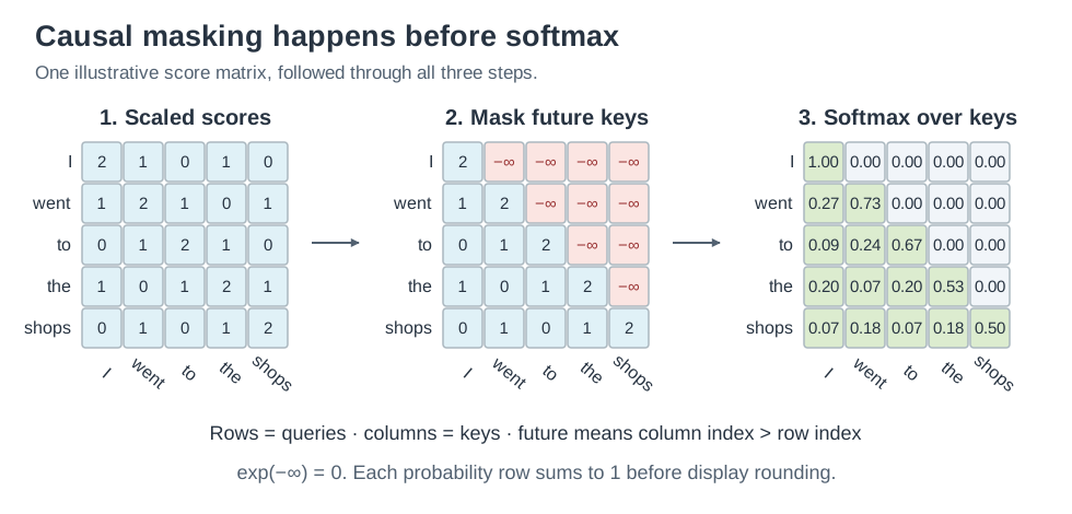
Follow the same illustrative scores across all three panels. Masked entries become zero probability; every row is normalized over its allowed keys. Values are rounded for display.
The toggle below compares the resulting access patterns for another sentence:
Each row is one token's attention distribution, produced bysoftmax(Q·Kᵀ / √d_k) and summing to 1; the output for that token is the weighted sum of every value vector using these weights. Switch toCausal and the upper triangle is masked to −∞ before the softmax, so a token can attend only to itself and the tokens before it — the surviving weights renormalize. The mask distinguishes bidirectional from causal attention. Implementations also differ in details such as normalization placement. Weights here are illustrative, chosen to show the shape of a real head, not dumped from a model.
For “the river bank,” the last row is unchanged: bank can already see the entire sequence. For “the bank river,” causal bank cannot receive anything from the future river position. The source restriction changed; the projection-and-mixing mechanism did not.
A mask specifies access, not a full positional encoding. Our position-free toy still has limitations; the block article explains where positional information enters. For generation, previously computed keys and values can be reused under causal attention—the KV-cache article follows that consequence. Cross-attention instead takes its queries and its key/value pairs from different sequences.
Watch real heads
The hand-set axes made arithmetic readable. In a trained model, inspect both where information is gathered and what contribution is produced.
BertViz visualizes attention patterns head by head. AttentionViz additionally supports exploring query/key geometry and patterns across inputs. exBERT is another exploration interface. These are companion tools, not evidence that a particular head must reproduce our toy.
Try two sentences containing different uses of bank. Inspect several heads and layers, then compare the corresponding hidden representations. A heatmap displays mixing coefficients; the values and output projection determine the vector actually contributed. Treat a proposed role such as “disambiguation head” as a hypothesis to test across inputs and with interventions.
Where this leaves us
We built a contribution in three stages: match, weight, mix. The initial bank experiment showed information flowing through a weighted sum. The Eiffel example separated matching from raw input similarity, and changing values showed that the same weights can carry different content. Training supplied the parameters instead of our hand choosing them.
The next step is to incorporate that contribution. In the simplest same-width case with identity output projection, tower = [1, 0] plus its swap-query mixture [0.2483, 0.5035] gives [1.2483, 0.5035]. The mixture is one contribution to an existing representation. A real block handles the output projection, multiple heads, normalization, and another update from the FFN.
Inside a transformer block follows those updates through the complete computation.
Optional: the mathematics behind the head
Theoretical and mathematical foundations
Learned matching, kernel smoothing, and memory
Substituting the projections into an unscaled score gives , with . Its rank is at most , and it need not be symmetric. This is a bilinear compatibility function, not generally a mathematical distance metric. The key distinction from raw similarity is the learned matrix between the two inputs.
The factorization is not unique: replacing by and by preserves the scores for invertible . This statement describes the plain content-only score; positional operations inserted between projections and scoring need separate treatment. Caching keys does not make the factors mathematically identifiable.
The normalized weighted sum also connects to kernel smoothing: use positive compatibility , normalize across sources, and average their values. Transformer Dissection develops this perspective. Hopfield Networks is All You Need connects an attention-style update to associative-memory retrieval. These are additional views of the operation, not prerequisites for running the toy.
There is a useful different mechanism if we remove softmax. With column vectors and constant scaling omitted, unnormalized causal linear attention can be rearranged as:
Update the memory by and read it with . The memory has fixed dimensions for fixed key/value widths. Linear Transformers Are Secretly Fast Weight Programmers relates this mechanism to earlier fast-weight systems. Standard softmax attention does not admit this rearrangement; removing softmax changes the operation.
Reverse-engineer a head you trained
A further experiment: repeated patterns and ablation
The companion examples/train_induction_head.py trains a two-layer attention-only model on repeated sequences, then measures attention patterns and ablates heads. This is a separate lab, beyond the one-head sense classifier. An induction pattern continues A B … A with B; the experiment tests whether the model discovers a mechanism useful for that task.
Run the script, record the loss and its induction scores, and compare loss before and after each ablation. Treat the existence and location of a particular circuit as a result to check, not as something guaranteed by the architecture or random seed. The script uses plain PyTorch; TransformerLens supplies hooks and activation access for more extensive investigations.
For a guided investigation, ARENA’s Introduction to Mechanistic Interpretability walks through finding induction heads, inspecting their QK and OV circuits, and testing their role with ablations using TransformerLens.
For a worked example before inspecting a trained model, skip-trigram bugs and induction heads shows why different queries can receive the same unwanted message, then builds a circuit that finds a continuation by matching the token that preceded it.
A name such as “coreference head” or “induction head” should summarize measured behavior. Correlation with a pattern suggests a role; intervention tests what depends on it. Even an ablation must be interpreted with care, since other components can interact with or compensate for the removed head.