A weight matrix acts on an entire activation vector produced by the previous layer, but we can understand its effect by examining the vector’s components. There are many ways to choose those components. The row-space and null-space decomposition gives us a precise split: one component produces the same output as the original input, while the other maps to zero. This explains how different activation vectors can produce exactly the same result.

Beyond the subspaces defined by a matrix, representation analysis and mechanistic interpretability also seek components associated with features, patterns, or particular computations. Finding directions that capture those features or computations is a discovery task: techniques such as PCA/SVD, linear probes, and sparse autoencoders identify candidates from data, whose meaning must be tested. The subspaces they span can differ from those defined by an individual weight matrix. Our focus here is the mathematical foundation—decomposing vectors and understanding matrix-defined subspaces—which prepares us to explore those learned representations.

In the previous article, we explored how weight matrices transform vectors and why neural networks need nonlinear activations. In this article, we’ll first explore how linear combinations build vectors, how vectors can be decomposed into components, and how a matrix transforms those components through dot products. Then we’ll introduce the null space and use it to understand the row space, before exploring the output geometry through the column space and left null space. We’ll work through small matrices, draw their spaces, and construct a projection that changes the input while preserving the next matrix’s output.

This article provides the linear algebra foundation for our MNIST experiment: what a trained classifier reads. In that experiment, a hidden layer produces a vector of 128 activation values for each handwritten digit image. We identify 118 independent directions that the trained output layer ignores, then remove the component along those directions while preserving its digit scores up to numerical roundoff. The null space tells us what we can remove, the row space describes what we keep, and projection performs that separation.

How a matrix transforms a vector’s components

A matrix defines a linear transformation from an input space to an output space. Its shape specifies the number of coordinates in those spaces; its entries determine where each input goes. In a neural network, the input space is the space in which activation vectors from the previous layer live. The output space is where the linearly transformed vectors live, before any nonlinear activation is applied.

To understand a matrix’s effect on a vector, we need to look at the vector components that it can be decomposed into. Each component is itself a vector in the input space, and the original vector is their sum. By linearity, the matrix transforms each component separately, and the resulting vectors add up to the same output as transforming the original vector directly. Some components may be stretched, shortened, or sent in a different direction, while others may map to zero and disappear entirely.

A vector has many possible decompositions, using coordinate axes or directions that cross several axes. In mechanistic interpretability and representation analysis, techniques such as PCA/SVD, linear probes, and sparse autoencoders help identify useful directions from data, revealing structure distributed across multiple entries of the activation vector.

Let’s now take a look at how to build a vector from components. Each option in the widget below builds the same blue vector $h=(5,3,2)$ using a different linear combination: each colored arrow is a chosen vector scaled by a coefficient, and these component vectors add up to $h$. The first option uses the three coordinate basis vectors $e_1=(1,0,0)$, $e_2=(0,1,0)$, and $e_3=(0,0,1)$. Each points along its corresponding coordinate axis and is scaled by the corresponding coordinate of $h$.

Coordinate basis Other basis Two vectors

(5, 3, 2) = 5(1, 0, 0) + 3(0, 1, 0) + 2(0, 0, 1)

Scale e₁

5

Scale e₂

3

Scale e₃

2

Let’s look more closely at the widget’s coordinate-basis option to distinguish a basis vector, its coefficient, and the resulting vector component. The basis vector $e_1$ is a unit vector representing a direction: it has length one. The scalar $5$ tells us how much to scale it, and $5e_1=(5,0,0)$ is the actual vector component. The three vector components add up to our input:

$$h=5e_1+3e_2+2e_3=(5,0,0)+(0,3,0)+(0,0,2)=(5,3,2).$$

Coordinates such as $5$ are often called scalar components. In this article, vector component means the whole scaled vector, such as $(5,0,0)$.

Separating direction from magnitude helps us reason about subspaces and transformations. Vectors such as $(1,1,1)$ and $(2,2,2)$ span the same line despite having different lengths. Representing their direction with a unit vector lets dot products measure signed projection lengths directly, and lets us examine how a matrix transforms that direction separately from how much of it is present in the input.

To make this separation explicit, we write a vector component as $\alpha d$: $d$ is a unit vector representing the chosen direction, and $\alpha$ is a signed scalar specifying how much of it to include. In our example, $d=e_1$ and $\alpha=5$. The component’s length is $|\alpha|$; a negative coefficient makes it point opposite to $d$.

How do we obtain this form when a component is given only by its coordinates? For any nonzero vector $v$, calculate its length $\|v\|$ and divide every coordinate by that length. This is normalization:

$$d=\frac{v}{\|v\|}, \qquad \alpha=\|v\|, \qquad v=\alpha d.$$

Choosing $d$ to point in the same direction as $v$ makes $\alpha$ positive. If we instead fix a unit direction first, a component pointing opposite to it has a negative coefficient.

We can demonstrate normalization using a vector already in the widget. One of the vectors in the “Other basis” set is $v=(1,1,1)$, which points across all three coordinate axes. Initially, its coefficient is $2$, so the green component is $2v=(2,2,2)$. These vectors have different lengths but the same direction.

To represent their shared direction with a unit vector, we could use L2 normalization. Normalization scales the vector to a total length of $1$ while preserving its direction. First, we calculate $v$‘s length by squaring its coordinates, adding them, and taking the square root. Then we divide every coordinate by that length. Scaling all coordinates by the same positive amount preserves the direction:

$$\|v\|=\sqrt{1^2+1^2+1^2}=\sqrt{3}, \qquad d=\frac{v}{\|v\|}=\frac{1}{\sqrt{3}}(1,1,1).$$

The resulting vector has length $\|d\|=\sqrt{\tfrac13+\tfrac13+\tfrac13}=1$. We can normalize any nonzero vector this way; the zero vector has no direction and cannot be divided by its length.

Multiplying by the original length reconstructs the basis vector: $v=\sqrt{3}\,d=(1,1,1)$. The widget’s green component can therefore be written as:

$$2v=2\sqrt{3}\,d =2\sqrt{3}\left(\frac{1}{\sqrt{3}},\frac{1}{\sqrt{3}},\frac{1}{\sqrt{3}}\right) =(2,2,2).$$

The coefficient is $2$ when we scale $v$, but $2\sqrt{3}$ when we scale the unit vector $d$. The component itself stays unchanged. Moving the first slider scales that component along the same direction; a negative value reverses it.

Let’s now look at how a matrix transforms those individual components. We have seen how to build $h$ by adding scaled vectors. When we apply a matrix $W$ to $h$, linearity lets us understand the result by transforming each component and adding the results: $Wh=Wv_1+Wv_2$ whenever $h=v_1+v_2$. Here, $Wv_1$ and $Wv_2$ are output vectors, which we add coordinate by coordinate.

Dot products

How does the matrix compute these contributions? Each row takes a dot product with the whole input vector, giving one coordinate of the output. We can break that scalar measurement into contributions from the individual vector components.

Start with the coordinate decomposition from the first widget:

$$h=c_1+c_2+c_3, \qquad c_1=(5,0,0),\quad c_2=(0,3,0),\quad c_3=(0,0,2).$$

For a single illustrative row $r=(2,1,3)$, linearity gives:

$$r\cdot h=r\cdot(c_1+c_2+c_3)=r\cdot c_1+r\cdot c_2+r\cdot c_3.$$

Each component supplies one scalar contribution to this output coordinate:

$$\begin{aligned} r\cdot c_1&=(2,1,3)\cdot(5,0,0)=10,\\ r\cdot c_2&=(2,1,3)\cdot(0,3,0)=3,\\ r\cdot c_3&=(2,1,3)\cdot(0,0,2)=6. \end{aligned}$$

Adding them gives $r\cdot h=10+3+6=19$, exactly the same result as computing $(2,1,3)\cdot(5,3,2)$ directly.

Geometrically, the row measures how much each component points along its direction, and adds those signed measurements. A raw dot product is a scalar, not a projection vector. For a nonzero row, write its unit direction as $\widehat r=r/\|r\|$. Then $r\cdot c=\|r\|(\widehat r\cdot c)$: the signed projection length of $c$ along the row, multiplied by the row’s length. The actual projection vector is $(\widehat r\cdot c)\widehat r$ and still lives in the input space. Matrix multiplication uses the scalar $r\cdot c$ as a contribution to one coordinate in the output space.

The components need not follow coordinate axes. For any component $c=\alpha d$, where $d$ is a unit vector, its contribution is:

$$\boxed{r\cdot c=r\cdot(\alpha d)=\alpha(r\cdot d).}$$

Here, $\alpha$ is the signed amount of that component in our chosen decomposition, while $r\cdot d$ tells us how strongly this row responds to a unit step along $d$. The contribution depends on both. A large component can contribute zero if its direction is perpendicular to the row. Contributions may also be positive or negative and can cancel one another.

For components associated with candidate features or patterns, this separates two questions: how much of a component is present in this input, and how does this row respond to its direction? The algebra applies to any exact decomposition; interpreting its components as meaningful features requires evidence. If the chosen components do not sum to the whole input, we must also include the remainder’s contribution.

Repeating the calculation for every row collects each component’s scalar contributions into an output vector, giving $Wh=Wc_1+Wc_2+Wc_3$. We can either sum component contributions within each row or transform each component into a vector and then add those vectors. Both compute the same output.

For the two-component split $h=v_1+v_2$ introduced above, each row $r$ gives:

$$r\cdot h=r\cdot v_1+r\cdot v_2.$$

This is the vector addition $Wh=Wv_1+Wv_2$ viewed one coordinate at a time. For a matrix with three rows, we can write out the whole output as:

$$Wh= \begin{pmatrix} r_1\cdot v_1+r_1\cdot v_2\\ r_2\cdot v_1+r_2\cdot v_2\\ r_3\cdot v_1+r_3\cdot v_2 \end{pmatrix}.$$

For example, the first output coordinate is $r_1\cdot h=r_1\cdot v_1+r_1\cdot v_2$: two scalar contributions added to produce one coordinate. Repeating this for every row produces the whole output vector. The vector equation shows how the transformed components add together; the dot products show how each coordinate is calculated.

So the calculation is equivalent to measuring each component separately and adding its contribution. The matrix doesn’t need to explicitly split the input first. If a component is perpendicular to every row, it contributes zero to every output coordinate and disappears under the transformation.

The next widget uses a different split of our example vector: $h=(5,3,2)=v_1+v_2$, with pink $v_1=(1,-1,0)$ and green $v_2=(4,4,2)$. Its matrix $W$ has rows $(1,1,0)$, $(0,0,1)$, and $(1,1,1)$. Here, $v_1$ is perpendicular to every row, so $Wv_1=0$:

$$Wh=Wv_1+Wv_2=0+Wv_2=Wv_2.$$

The $0$ here means the zero vector $(0,0,0)$. For this example, the coordinate-by-coordinate addition is:

$$Wh=(0,0,0)+(8,2,10)=(8,2,10).$$

Only $v_1$‘s contribution disappears; the output comes entirely from $v_2$. If $v_1$ is perpendicular to just one row, its contribution to that row’s output coordinate is zero, but it may contribute to the others.

In the widget, each row’s dot product gives one output coordinate. The calculation underneath separates the contributions from pink $v_1$ and green $v_2$, so you can see why the pink component contributes zero throughout.

W =

110001111

h =

532

Wh =

8210

h = (5, 3, 2) = (1, −1, 0) + (4, 4, 2)

Pink v₁ is perpendicular to every row. Green v₂ supplies the output. The blue input is h = v₁ + v₂.

r₁ · h = (1, 1, 0) · (5, 3, 2) = 8

r₁ · v₁ + r₁ · v₂ = 0 + 8 = 8

r₂ · h = (0, 0, 1) · (5, 3, 2) = 2

r₂ · v₁ + r₂ · v₂ = 0 + 2 = 2

r₃ · h = (1, 1, 1) · (5, 3, 2) = 10

r₃ · v₁ + r₃ · v₂ = 0 + 10 = 10

Input h₁

5

Input h₂

3

Input h₃

2

Add (1, −1, 0)Try a null-space inputReset

Try Add (1, −1, 0): the input changes, but every output coordinate stays the same. Try a null-space input makes the entire output zero. One row’s dot product with the whole input being zero makes only that output coordinate zero; all three must be zero for the whole output to vanish.

This brings us from individual components to subspaces: entire sets of vectors with a shared structure. All input vectors perpendicular to every row of $W$ form its null space. Every vector in this subspace maps to zero, just like our pink component. Its perpendicular complement in the input space is the row space, which contains our green component.

This is how a matrix can erase part of an input while still producing a nonzero output. When we split the input into its row-space and null-space components,

$$h=h_{\mathrm{row}}+h_{\mathrm{null}} \quad\Longrightarrow\quad Wh=Wh_{\mathrm{row}}+0.$$

The null-space component disappears, while a nonzero row-space component still produces an output. The matrix can also change the surviving component’s length and direction. Erasing a component of the input is different from mapping the entire input to zero: only an input lying entirely in the null space is erased completely.

How linear combinations and dot products connect

A linear combination constructs a vector; a dot product measures a vector along one particular direction. These give us two complementary ways to understand the transformation we have just explored.

Given vectors $v_1$ and $v_2$, we can choose coefficients $a$ and $b$ and construct $x=av_1+bv_2$. Varying those coefficients reaches every vector in their span. If the two vectors are independent, that span is a plane through the origin.

A dot product starts with a vector $x$ and measures it against another vector $v$, producing one scalar $x\cdot v$. If $v$ has length one, this is the signed length of $x$‘s projection along $v$‘s direction. For a nonzero vector of any length,

$$x\cdot v=\|v\|\left(x\cdot\frac{v}{\|v\|}\right).$$

So the dot product also scales that signed projection length by $\|v\|$. The result is a scalar measurement, not a projection vector. For a unit vector $v$, the projection vector is $(x\cdot v)v$: we use the scalar to scale the direction vector.

Can dot products recover the coefficients used to build a vector? Yes, directly when the basis is orthonormal: its vectors are perpendicular to one another and each has length one. For example, take $v_1=(1,0)$, $v_2=(0,1)$, and $x=3v_1+2v_2=(3,2)$. Dotting $v_1$ with the resulting vector $x$ gives:

$$v_1\cdot x =v_1\cdot(3v_1+2v_2) =3(v_1\cdot v_1)+2(v_1\cdot v_2) =3(1)+2(0)=3.$$

The perpendicular component contributes zero, so we recover exactly the coefficient of $v_1$. Similarly, $v_2\cdot x=2$. For an orthonormal basis $v_1,\ldots,v_n$, this gives the reconstruction formula:

$$x=\sum_{i=1}^{n}(x\cdot v_i)v_i.$$

Linear combination takes coefficients to a vector; dot products with an orthonormal basis take the vector back to its coefficients. If the orthonormal vectors span only a subspace, the same sum reconstructs the projection of $x$ onto that subspace. It equals all of $x$ only when $x$ lies in that span.

This qualification matters for our widget. Dot products with the Coordinate basis recover the coefficients $5,3,2$. With Other basis, the vectors are not orthogonal, so dotting with them mixes contributions from several components. To recover the coefficients, we must solve the corresponding linear system or take dot products with a dual basis—vectors chosen to return one for their matching basis vector and zero for the others. If a basis is orthogonal but its vectors are not unit length, dividing each dot product by the squared length is enough: $a_i=(x\cdot v_i)/(v_i\cdot v_i)$.

Normalization rewrites a vector we already have as a length times a unit direction. To find the component of another vector $h$ along a chosen unit direction $d$, we can use orthogonal projection. The dot product gives its signed amount, $\alpha=h\cdot d$. Using the normalized direction $d=(1,1,1)/\sqrt{3}$ from Other basis and $h=(5,3,2)$:

$$\alpha=\frac{5+3+2}{\sqrt{3}}=\frac{10}{\sqrt{3}}, \qquad \alpha d=\left(\frac{10}{3},\frac{10}{3},\frac{10}{3}\right).$$

The remainder is $h-\alpha d=(5/3,-1/3,-4/3)$, which is perpendicular to $d$. This projection component differs from the widget’s green component $(2,2,2)$: projection chooses a perpendicular remainder, while the widget’s Other basis uses a non-orthogonal basis. Both decompositions add up to the same $h$, but their components differ. The coefficients of a non-orthogonal basis are not generally given by dotting the result with its basis vectors.

In representation analysis, we may look for components associated with particular features or patterns rather than coordinate axes. If a unit vector $d$ represents a candidate feature direction, it can involve many activation coordinates together. For a particular activation vector $h$, its projection component is $(h\cdot d)d$: $d$ specifies the direction, while the scalar $h\cdot d$ depends on the input. Whether that direction captures the proposed feature still needs to be tested.

This connects directly to a neural network’s weight matrix. If the rows of $W$ are $w_1^T,\ldots,w_m^T$, then:

$$Wx=\begin{pmatrix}w_1\cdot x\\\vdots\\w_m\cdot x\end{pmatrix}.$$

Each nonzero row measures the input along its learned direction, scaled by that row’s length. The output collects these scalar measurements into a vector. The rows need not point in different directions or form an orthonormal basis, so these outputs are not generally coefficients that reconstruct the input using the rows themselves.

We can also read the same multiplication through the columns. If $W$ has columns $c_1,\ldots,c_n$, then:

$$Wx=x_1c_1+\cdots+x_nc_n.$$

The rows measure the input through dot products; the columns construct the output through a linear combination. Both describe exactly the same matrix multiplication. The row directions live in the input space, while the column vectors live in the output space. If the rows form a full orthonormal basis of the input space, we can reconstruct the input from the measurements: $x=\sum_i(w_i\cdot x)w_i=W^T(Wx)$. Otherwise, that simple reconstruction is not guaranteed.

Thinking in terms of these measurements and contributions makes the transformation view more concrete: $W$ transforms the whole vector, and dot products and linear combinations show how that computation works.

Understanding a transformation through its subspaces

A set of directions spans a subspace—all the vectors we can build by scaling and adding vectors along those directions. This lets us describe whole sets of possible components, rather than one input at a time. The row space and null space describe the input side of a matrix transformation; the column space and left null space describe the output side. We’ll explore all four, with a focus on the null space.

Usually we want to know which vectors in the output space we can reach by varying a vector in the input space. For these constructions, the input vector $x$ contains the coefficients controlled by the sliders, and the output vector is $h$. Put the construction vectors into the columns of a matrix $A$, so that $Ax=h$. The output space is $\mathbb R^3$ in all three widget options, because $h$ has three coordinates. The column space tells us which part of that output space is reachable.

The diagram below shows the four fundamental subspaces defined by the layer’s weight matrix: the row space and null space divide the input space into perpendicular parts, while the column space contains every possible output and the left null space is perpendicular to it.

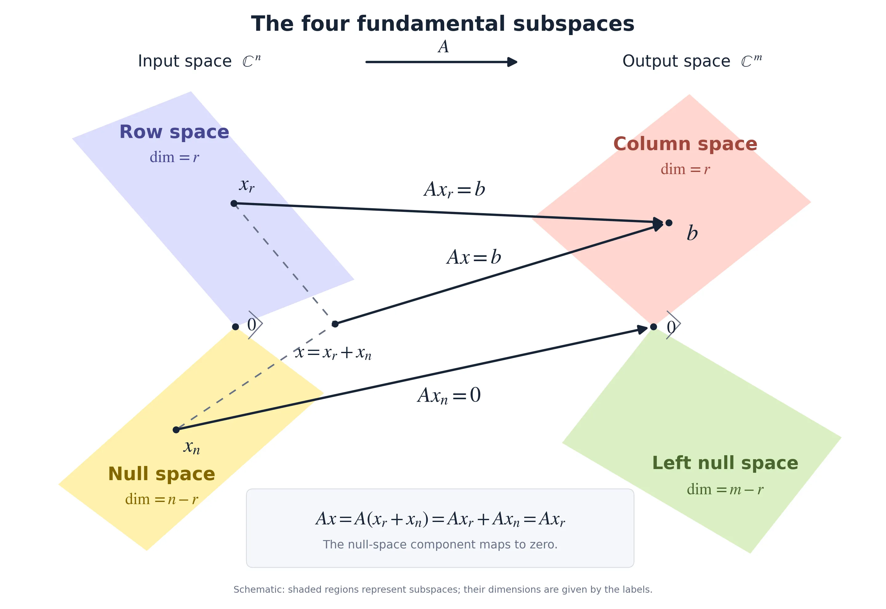
The image uses $A$ for our matrix $W$, $x$ for our input $h$, and $b$ for the output of the matrix multiplication—not an added bias term. It labels the spaces over $\mathbb{C}$; our examples use real-valued vectors in $\mathbb{R}$. The fourth subspace, the left null space, is perpendicular to the column space in the output space.

For Coordinate basis, the construction is:

$$A=\begin{pmatrix}1&0&0\\0&1&0\\0&0&1\end{pmatrix}, \qquad x=\begin{pmatrix}5\\3\\2\end{pmatrix}, \qquad Ax=\begin{pmatrix}5\\3\\2\end{pmatrix}.$$

In a neural network, we can view $A$ as a layer’s weight matrix and $x$ as the activation vector produced by the previous layer. The matrix transforms that input vector into the output vector $Ax$. Here, $A$ is the identity matrix, so it leaves the activations unchanged. In the widget, the sliders supply the values of $x$; in a network, the previous layer computes them.

The input space is $\mathbb R^3$, with one coefficient for each of the three columns. Those columns are independent, so the column space fills the entire output space $\mathbb R^3$: every output vector is reachable.

The three rows are also linearly independent, so the row space fills the entire input space $\mathbb R^3$: the matrix ignores no input direction. The row space describes the input side, while the column space describes the reachable output side. The number of independent rows always equals the number of independent columns—the matrix’s rank. Here, that rank is 3.

For Other basis, we use different columns and coefficients:

$$A=\begin{pmatrix}1&1&2\\1&-1&2\\1&1&-1\end{pmatrix}, \qquad x=\begin{pmatrix}2\\1\\1\end{pmatrix}, \qquad Ax=\begin{pmatrix}5\\3\\2\end{pmatrix}.$$

The input space and output space are both still $\mathbb R^3$. These three columns are also independent, so their column space fills the entire output space. We changed the construction vectors and input coefficients, but can still reach every output vector.

For Two vectors, the matrix has only two columns:

$$A=\begin{pmatrix}4&1\\1&2\\1&1\end{pmatrix}, \qquad x=\begin{pmatrix}1\\1\end{pmatrix}, \qquad Ax=\begin{pmatrix}5\\3\\2\end{pmatrix}.$$

The input space is now $\mathbb R^2$, because we supply only two coefficients. The output space remains $\mathbb R^3$, but the two independent columns span only a plane within it. That plane is the column space: we can reach $h=(5,3,2)$ because it lies there, but output vectors outside it are unreachable.

Widget option	Input space: coefficients $x$	Reachable part of the output space: column space
Coordinate basis	$\mathbb R^3$	All of $\mathbb R^3$
Other basis	$\mathbb R^3$	All of $\mathbb R^3$
Two vectors	$\mathbb R^2$	A plane inside $\mathbb R^3$

In all three examples, the columns are independent, so the row space fills the entire input space, and the null space contains only the zero input vector. These reachable output spaces assume arbitrary real input coefficients; the widget’s integer sliders show only some examples within them.

Input and output are roles relative to a particular matrix. Here, $h$ lives in the output space of the construction matrix $A$. When we apply the layer’s weight matrix $W$, that same $h$ lives in its input space, and $Wh$ lives in its output space.

For the weight matrix $W$, the row space and null space give us a particular way to split $h$: one component lies in the row space, and the other lies in the null space. The matrix transforms the row-space component and maps the null-space component to zero. The subspaces describe where these components lie; the matrix performs the transformation. Either component can be zero, in which case the whole input lies in the other subspace.

The central relationship is that any input splits into a row-space component and a null-space component. The matrix maps the null-space component to zero, so the whole input and its row-space component reach the same output:

$$Wh=W(h_{\mathrm{row}}+h_{\mathrm{null}})=Wh_{\mathrm{row}}, \qquad Wh_{\mathrm{null}}=0.$$

In this discussion, when we say “given a vector” without specifying a space, we mean a vector in the input space: $(a,b)$ for a two-coordinate input, or $(a,b,c)$ for our three-coordinate example. We then ask what the matrix does to it and whether it belongs to the row space or null space. This is a convention for our explanation; the coordinate notation alone does not distinguish an input from an output. We write the resulting output as $Wh$ or $z$.

The widget starts with the Original $3\times3$ matrix, which maps $h$ to $(h_1+h_2,\;h_3,\;h_1+h_2+h_3)$. It returns three numbers, but the third is the sum of the first two, so every output lies in a two-dimensional column-space plane. The row space is a plane in the input space, and the null space is the perpendicular line in direction $(1,-1,0)$. Choose Alternative to compare a matrix with a row-space line and a null-space plane. Switching matrices keeps your input vector, so you can see how its decomposition changes. The four subspace explanations below use Original; the rank comparison then works through Alternative. The separate plane-construction animation also uses the Original matrix.

One matrix, four subspaces

Choose a matrix, then change the input vector. Each matrix fixes its own four subspaces.

Choose the matrix

Original · row plane, null line Alternative · row line, null plane

W =

110001111

3 inputs → 3 outputs · rank 2Wh = (h₁ + h₂, h₃, h₁ + h₂ + h₃)The third output is the sum of the first two.

Input dimensions: row space 2 + null space 1 = 3. Output dimensions: column space 2 + left null space 1 = 3.

Input space · ℝ³

Row space: h₁ = h₂ · plane
Null space: (d, −d, 0) · line

Output space · ℝ³

Column space: z₃ = z₁ + z₂ · plane
Left null space: (−d, −d, d) · line

Drag either 3D view to rotate it, or focus it and use the arrow keys. The blue and green output arrows overlap because Wh = Whrow.

Input h₁

5

Input h₂

3

Input h₃

2

Add (1, −1, 0)Remove null componentTry a null-space vectorReset

Show matrix row and column vectors Show left null space

The input lies outside both the row-space plane and the null-space line. It has a component in each.

Whole input h(5, 3, 2)W → (8, 2, 10)

Row-space component hrow(4, 4, 2)W → (8, 2, 10)

Null-space component hnull(1, −1, 0)W → (0, 0, 0)

The green plane and pink line split the input space. The orange plane contains every possible output. The purple line is perpendicular to that plane: it is the null space of Wᵀ, not a destination for inputs erased by W. Those inputs map to the origin.

Rotate either view and change the input coordinates. Then try Add (1, −1, 0) or Remove null component: the input changes, but the output stays fixed. A vector entirely in the null space maps to the origin. Its destination is not the left null space, which is a separate subspace defined by $W^\top$.

The other subspaces help explain this operation: row space describes the component we keep, and column space describes all possible outputs of the weight matrix. Rank counts the independent directions in each of these two spaces. Together, these ideas explain why different input vectors can produce the same output.

Reading the arrows in the Original view

Blue vector: the whole input $h$. In the input plot, it is the sum of the green row-space component and the pink null-space component: $h = h_{\mathrm{row}} + h_{\mathrm{null}}$. This is a linear combination with both coefficients equal to 1.

Green vector: the component $h_{\mathrm{row}}$ lying in the row-space plane. Move the pink arrow so its tail starts at the green arrow’s tip, and it reaches the blue arrow’s tip. The dashed lines show this addition.

Pink vector: the component $h_{\mathrm{null}}$ lying on the null-space line. Applying $W$ maps it to zero, so its output is the origin, with no arrow length.

One visible output arrow: the blue and green output arrows overlap because $Wh = Wh_{\mathrm{row}} + Wh_{\mathrm{null}} = Wh_{\mathrm{row}}$. This is the output for the currently selected input; changing the input can move it within the orange column-space plane.

In the input plot, the pink (red) vector is exactly the difference between blue and green: $h-h_{\mathrm{row}}=h_{\mathrm{null}}$. If that component were zero, blue and green would overlap in the input plot too. Applying $W$ sends their difference to zero, so their outputs overlap even when the inputs differ. This happens for every matrix when we split the input into that matrix’s row-space and null-space components.

The companion MNIST experiment applies this geometry to a trained network: its full hidden space has 128 dimensions, its output matrix has a 10-dimensional row space, and its null space has 118 dimensions. Here, we first build the geometry with matrices small enough to inspect and draw.

Null space: which input changes leave the output unchanged?

The null space is our starting point because we want to know what we can remove from an input without changing the output. If a vector $n$ satisfies $Wn=0$, adding or removing it has no effect on the matrix’s output:

$$W(h+n)=Wh+Wn=Wh.$$

The matrix $W$ determines its subspaces. Once we fix the matrix, they stay fixed as the input changes. We’ll use the widget’s Original matrix:

$$W=\begin{bmatrix}1&1&0\\0&0&1\\1&1&1\end{bmatrix}.$$

We find the null space by asking: which inputs does $W$ send to zero? For an input with coordinates $(x,y,z)$, the matrix produces:

$$W\begin{bmatrix}x\\y\\z\end{bmatrix} =\begin{bmatrix}x+y\\z\\x+y+z\end{bmatrix}.$$

Set every output coordinate to zero:

$$x+y=0,\qquad z=0,\qquad x+y+z=0.$$

The first two equations give $y=-x$ and $z=0$. The third equation is then automatically satisfied, so it adds no further restriction. Every null-space vector therefore looks like:

$$(x,-x,0)=x(1,-1,0).$$

Only one number, $x$, is free to change. Every possible vector is a multiple of the same direction $(1,-1,0)$, so their tips trace a line through the origin. For example, $(1,-1,0)$, $(2,-2,0)$, and $(-1,1,0)$ all lie on that line, and all map to zero.

Calling the free coefficient $d$, as in the widget, we can write the whole null space as:

$$\operatorname{Null}(W)=\{d(1,-1,0):d\in\mathbb{R}\}.$$

Changing $d$ moves along the red line. This line is determined by $W$ and stays fixed when we change the input. It describes the differences this output layer cannot detect. We can now ask what remains when we remove that component: this leads us to the green row-space plane.

Row space: which combinations of inputs does the matrix measure?

For a real matrix, the row space is the perpendicular complement of the null space:

$$\operatorname{Row}(W)=\operatorname{Null}(W)^\perp.$$

Given a vector $(a,b,c)$ and the null-space direction $(1,-1,0)$ we just found, we have enough information to determine whether that vector belongs to the row space. It must be perpendicular to the null-space direction, so we check its dot product:

$$(a,b,c)\cdot(1,-1,0)=a-b=0.$$

This requires $a=b$, while $c$ can be anything. We have therefore recovered the entire row space directly from the null space:

$$\operatorname{Row}(W)=\{(a,a,c):a,c\in\mathbb{R}\}.$$

That’s the green plane $h_1=h_2$. Once we know which directions the matrix erases, we can identify its row space as all input vectors perpendicular to those directions. Here the null space is a line, so checking its one basis direction is enough; for a larger null space, we would check perpendicularity to every vector in a basis.

To see the connection, recall that each output coordinate is a dot product with one row of $W$. If $Wn=0$, every row has zero dot product with $n$. Every linear combination of the rows is therefore perpendicular to every null-space vector. The row space contains all the input directions perpendicular to the null space; within it, distinct vectors produce distinct outputs. The matrix can still scale or redirect these vectors.

Read one row to understand one output coordinate

A matrix’s shape is written as rows by columns. The widget has three input coordinates and three output coordinates, so its matrix is $3\times3$: three rows, each containing three weights. To understand how the first output coordinate is produced, read the first row; the second and third rows produce the other two output coordinates.

Row vectors live in the input space. Each has three coordinates and tells us how to combine the input values to calculate exactly one output coordinate.

The three rows are:

$$r_1=(1,1,0),\qquad r_2=(0,0,1),\qquad r_3=(1,1,1).$$

Each row takes a dot product with the input: multiply corresponding coordinates and add the results. Together, the three dot products give

$$Wh=\begin{bmatrix}r_1\cdot h\\r_2\cdot h\\r_3\cdot h\end{bmatrix} =\begin{bmatrix}h_1+h_2\\h_3\\h_1+h_2+h_3\end{bmatrix}.$$

We can read those calculations one output at a time:

Row	Output coordinate	What happens to the input values
$(1,1,0)$	$z_1=h_1+h_2$	Include $h_1$ and $h_2$ unchanged, then add them; $h_3$ contributes nothing to this output.
$(0,0,1)$	$z_2=h_3$	Include $h_3$ unchanged; $h_1$ and $h_2$ contribute nothing to this output.
$(1,1,1)$	$z_3=h_1+h_2+h_3$	Add all three input values; this output is the sum of the first two.

Our matrix scales and combines these values to produce each output coordinate—a linear combination. The weights determine their contributions:

• A weight of 0 ignores that input value for this output.
• A weight of 1 includes it unchanged.
• Other weights scale it, with negative weights reversing its sign.
• Several nonzero weights combine several input values into one output.

For example, if we changed the first row to $(3,1,0)$, the first output would become $3h_1+h_2$: the contribution from $h_1$ would be tripled, the contribution from $h_2$ would stay unchanged, and $h_3$ would still contribute nothing to that output. These weights determine the contributions to the new output coordinate; they do not modify the stored input values themselves. Our running example keeps the original row $(1,1,0)$.

A zero in one row does not mean the whole transformation drops that input coordinate. Here, the first row ignores $h_3$, but the second row uses it. A direction is fully silenced only when every row has a zero dot product with it. For $(1,-1,0)$, the first row gives $1-1=0$, the second gives $0$, and the third gives $1-1+0=0$. That direction therefore lies in the matrix’s null space, even though both $h_1$ and $h_2$ contribute to the first output.

From individual rows to the row-space plane

The row space contains all linear combinations of the matrix’s rows. Here the third row is the sum of the first two: $(1,1,1)=(1,1,0)+(0,0,1)$. It is linearly dependent on them, so it adds no new direction. We can leave it out when determining the row space: the first two rows are linearly independent and already span the entire plane. The third row still participates in the matrix multiplication, producing the third output coordinate, which is always the sum of the first two outputs.

Let’s calculate that space explicitly. Every vector in the row space is a linear combination of the rows. Since $r_3=r_1+r_2$, we can rewrite any such combination using just the first two:

$$\begin{aligned} \alpha r_1+\beta r_2+\gamma r_3 &=\alpha r_1+\beta r_2+\gamma(r_1+r_2)\\ &=(\alpha+\gamma)r_1+(\beta+\gamma)r_2. \end{aligned}$$

Call those two coefficients $a=\alpha+\gamma$ and $b=\beta+\gamma$. Then:

$$\begin{aligned} a(1,1,0)+b(0,0,1) &=(a,a,0)+(0,0,b)\\ &=(a,a,b). \end{aligned}$$

Allowing $a$ and $b$ to be any real numbers gives the entire row space:

$$\operatorname{Row}(W)=\{(a,a,b):a,b\in\mathbb{R}\}.$$

That’s the green plane: its vectors’ first two coordinates must be equal, so its equation is $h_1=h_2$. Changing $a$ and $b$ lets us reach every point in that plane.

These vectors have three coordinates because they live in 3D input space, but there are only two independent choices: $a$ sets the first two coordinates together, and $b$ sets the third. That’s why the row space is a 2D plane inside 3D space. The green vector’s tail stays at the origin, while its tip can move anywhere within the plane $h_1=h_2$. Think of a sheet of paper in a room: every point on the sheet has three room coordinates, but movement along the sheet has only two independent directions.

Build the row-space plane

Two independent row vectors give us two directions to move: r₁ = (1, 1, 0) and r₂ = (0, 0, 1).

1. Start with two vectors2. Extend the first into a line3. Move the line to fill a plane

The blue row vector points diagonally in the h₁–h₂ plane. The orange row vector points along h₃.

0(1, 1, 0) + 0(0, 0, 1) = (0, 0, 0)

Play animationResetAnimation progress

Drag the view to rotate it, or focus it and use the arrow keys. Play the animation or move the timeline yourself.

The green arrow is one example of the sum a r₁ + b r₂ = (a, a, b). Its tip lies on the plane. Every point we reach has h₁ = h₂, while h₃ is unrestricted. The drawing shows a finite patch; allowing all real a and b fills the infinite row-space plane.

A span is one way to describe a subspace: give a set of vectors and take all their linear combinations. For example,

$$S=\operatorname{span}\{v_1,v_2\} =\{av_1+bv_2:a,b\in\mathbb{R}\}.$$

We can also describe the same subspace using conditions its vectors must satisfy. For our row-space plane, these two descriptions are equivalent:

$$\operatorname{row}(W) =\operatorname{span}\{(1,1,0),(0,0,1)\} =\{h\in\mathbb{R}^3:h_1=h_2\}.$$

The span tells us how to build every vector in the plane. The equation tells us whether a vector belongs to it. We do not have to start with a spanning set to define a subspace. For the null space, we start with the condition $Wn=0$ and solve it to find vectors that span all the solutions.

Do we calculate the two spaces differently? For the row space, the matrix already gives us vectors that span it: its rows. We find an independent set of rows that spans the same space to get a basis. For the null space, we solve the linear system $Wh=0$, then express its solutions using free variables to obtain a basis. In our example, the row-space basis is $(1,1,0)$ and $(0,0,1)$, while the null-space basis is $(1,-1,0)$.

Finding independent rows can also require calculation. Our example was easy because we could immediately see $r_3=r_1+r_2$. For larger matrices, row reduction helps with both tasks: the nonzero rows of a row-echelon form give a basis for the same row space, and the reduced equations let us solve for the null space.

Splitting an input into its row-space and null-space components

The two subspaces together cover the entire input space. For a real matrix with $n$ input coordinates:

$$\mathbb{R}^n=\operatorname{Row}(W)\oplus\operatorname{Null}(W).$$

Here $\oplus$ means every input has exactly one decomposition $h=h_{\mathrm{row}}+h_{\mathrm{null}}$, with one component in each subspace. The components are perpendicular, and applying the matrix gives:

$$Wh=W(h_{\mathrm{row}}+h_{\mathrm{null}}) =Wh_{\mathrm{row}}+\underbrace{Wh_{\mathrm{null}}}_{0} =Wh_{\mathrm{row}}.$$

This is the relationship our projection will use: the row-space component determines the scores, while the null-space component contributes zero. The row space need not contain the whole input for the matrix to produce a nonzero output.

You know you can build blue from green and red (pink in the widget) through a linear combination, so you’d expect to adjust green or red and watch blue change. That would work.

The widget runs that process backward: you choose blue, and it finds the green and red vectors that add up to it. This is called decomposition.

Normally, that would be ambiguous: many pairs of vectors add up to the same blue vector. But here there are restrictions:

• Green must lie in the fixed row-space plane.
• Red must lie on the fixed null-space line, perpendicular to that plane.

Blue can lie anywhere in the input space. We’re asking for a green vector in this matrix’s row space and a red vector in its null space whose sum is blue. Because the plane and line are perpendicular and together cover the input space, those restrictions leave exactly one pair for each blue vector. For the default input, that pair is $(4,4,2)+(1,-1,0)=(5,3,2)$.

How do we calculate that pair? If green and red are already known, blue is simply their sum. For the Original matrix, the constraints give green the form $(a,a,b)$ and red the form $(d,-d,0)$. Adding them gives:

$$h=(a,a,b)+(d,-d,0)=(a+d,\;a-d,\;b).$$

For example, choosing $a=4$, $b=2$, and $d=1$ gives $(4,4,2)+(1,-1,0)=(5,3,2)$.

The widget calculates backward. You supply blue, $h=(h_1,h_2,h_3)$, and it matches the coordinates of that sum to your input:

$$a+d=h_1,\qquad a-d=h_2,\qquad b=h_3.$$

Adding the first two equations gives $2a=h_1+h_2$. Subtracting the second from the first gives $2d=h_1-h_2$. Therefore:

$$a=\frac{h_1+h_2}{2},\qquad d=\frac{h_1-h_2}{2},\qquad b=h_3.$$

Substitute these values into the two component vectors:

$$h_{\mathrm{row}}=\left(\frac{h_1+h_2}{2},\frac{h_1+h_2}{2},h_3\right), \qquad h_{\mathrm{null}}=\left(\frac{h_1-h_2}{2},-\frac{h_1-h_2}{2},0\right).$$

For blue $=(5,3,2)$, these formulas give $a=4$, $d=1$, and $b=2$: green $=(4,4,2)$ and red $=(1,-1,0)$. Changing an input coordinate makes the widget recalculate these same formulas.

Blue lies in the row-space plane only when its red component is zero. Clicking Remove null component makes blue and green the same vector. Changing the input coordinates recalculates the two components; the matrix and its subspaces stay fixed.

The same idea also helps when solving an equation such as $Wh=z$. Once we have one solution $h_0$, all inputs producing that same output have the form $h_0+n$, where $n$ belongs to the null space. For a neural network’s linear layer, these are different representations that the layer cannot distinguish.

Column space: which outputs can the matrix produce?

Column vectors live in the output space. Each has three coordinates and tells us where an input basis vector goes. Their span is called the column space: the set of all possible linear combinations of the column vectors, which gives us all possible outputs $Wh$.

For our matrix, the three columns are:

$$c_1=\begin{bmatrix}1\\0\\1\end{bmatrix},\qquad c_2=\begin{bmatrix}1\\0\\1\end{bmatrix},\qquad c_3=\begin{bmatrix}0\\1\\1\end{bmatrix}.$$

Let $e_1=(1,0,0)$, $e_2=(0,1,0)$, and $e_3=(0,0,1)$ be the input basis vectors. Then $We_1=c_1$, $We_2=c_2$, and $We_3=c_3$. Multiplication builds the output by scaling and adding these columns:

$$Wh=h_1c_1+h_2c_2+h_3c_3.$$

All linear combinations of the columns form the column space. Since $c_2=c_1$, every output has the form:

$$s(1,0,1)+t(0,1,1)=(s,t,s+t).$$

This is the orange plane $z_3=z_1+z_2$ in the widget. The output has three coordinates, but only two can vary independently.

Three column vectors do not imply a three-dimensional span. The second column adds no new direction, while $c_1$ and $c_3$ are independent. They form a basis for this two-dimensional column space. The number of independent directions determines the dimension of a span, not the number of vectors in the list.

Rows and columns give two ways to calculate exactly the same transformation:

	Columns	Rows
Where the vectors live	Output space, $\mathbb{R}^3$	Input space, $\mathbb{R}^3$
Role in multiplication	Combine to build the output	Each computes one output coordinate
Their span	Column space: all possible outputs	Row space: all linear combinations of the row vectors

Both spans have dimension 2, but they occupy separate spaces: the input plane is $h_1=h_2$, while the output plane is $z_3=z_1+z_2$. The matrix accepts inputs from all of $\mathbb{R}^3$, including vectors outside its row space, and sends every one of them into its column space.

Left null space: which output directions are perpendicular to every possible output?

The fourth subspace also lives in the output space. The left null space is the null space of $W^\top$: vectors $q$ satisfying $W^\top q=0$. Equivalently, they are perpendicular to every column of $W$, and therefore to every output $Wh$.

For the Original matrix, let $q=(q_1,q_2,q_3)$. Then:

$$W^\top q= \begin{bmatrix} q_1+q_3\\ q_1+q_3\\ q_2+q_3 \end{bmatrix}=0.$$

These equations give $q_1=q_2=-q_3$, so the left null space is the purple line:

$$q=d(-1,-1,1),\qquad d\in\mathbb{R}.$$

It is perpendicular to the orange column-space plane. You can check this for any output $(s,t,s+t)$:

$$(-1,-1,1)\cdot(s,t,s+t)=-s-t+(s+t)=0.$$

The left null space is not where erased inputs go. The pink input null-space component maps to the origin. The purple line describes directions perpendicular to all possible outputs of the matrix multiplication. The widget’s Show left null space toggle lets you inspect it separately.

Bases and rank: how many independent directions are there?

A basis gives us a compact description of a subspace: an independent set of vectors whose linear combinations produce every vector in it. For the Original matrix, the first two rows form a basis for the row-space plane, and the columns $c_1$ and $c_3$ form a basis for the column-space plane. The third row and second column add no new directions.

The matrix’s rank is the dimension of its column space or, equivalently, its row space. These dimensions are equal for every matrix. Our Original matrix has rank 2: both spaces have two independent directions. Rank counts independent directions, not the total number of columns or rows.

Can the null space be a plane instead? Choose Alternative in the four-subspaces widget. It uses:

$$W_{\mathrm{alt}}=\begin{bmatrix}1&1&0\\2&2&0\\3&3&0\end{bmatrix}.$$

All three rows are multiples of $(1,1,0)$, so their linear combinations trace a row-space line. To find the null space, set the output to zero:

$$W_{\mathrm{alt}}\begin{bmatrix}x\\y\\z\end{bmatrix} =\begin{bmatrix}x+y\\2(x+y)\\3(x+y)\end{bmatrix} =\begin{bmatrix}0\\0\\0\end{bmatrix}.$$

All three equations require only $y=-x$; $z$ can be anything. Every null-space vector therefore has the form:

$$(x,-x,z)=x(1,-1,0)+z(0,0,1).$$

Two free numbers give a null-space plane. Try Add (0, 0, 1): the input’s third coordinate changes, but the output stays fixed. For the default input $(5,3,2)$, the new decomposition is $(4,4,0)+(1,-1,2)$, and both the whole input and its row-space component map to $(8,16,24)$.

Input subspace	Original matrix	Alternative matrix
Row space	Plane (2D)	Line (1D)
Null space	Line (1D)	Plane (2D)

If one is a plane in our 3D input space, the other must be a line. The row-space dimension is the matrix’s rank, and the row-space and null-space dimensions always add up to the number of input coordinates. This is the rank–nullity theorem:

$$\dim\operatorname{Row}(W)+\dim\operatorname{Null}(W)=3.$$

Neither space must always be a line. These are all the possibilities for three input coordinates:

Row space	Null space
3D space	Only the zero vector (0D)
Plane (2D)	Line (1D)
Line (1D)	Plane (2D)
Only the zero vector (0D)	3D space

With four input coordinates, both spaces could be 2D planes inside $\mathbb{R}^4$. It’s the number of independent directions that matters.

The output geometry changes too: the alternative matrix produces only multiples of $(1,2,3)$, so its column space is a line. Its left null space is the perpendicular plane $z_1+2z_2+3z_3=0$. Inputs erased by either matrix still map to the origin.

Simplify to two outputs to build a projection

To build the projection by hand, we’ll return to the Original matrix and simplify it to $2\times3$ by dropping the redundant third output. The row space and null space stay the same; the outputs now have two coordinates and fill all of $\mathbb{R}^2$. Its left null space then contains only the zero vector.

Part of the simplified transformation	Our small example
Output matrix $W$	$\begin{bmatrix}1&1&0\\0&0&1\end{bmatrix}$
Original vector $h$	$(5,3,2)$
Row-space component $h_{\mathrm{row}}$	$(4,4,2)$
Null-space component $h_{\mathrm{null}}$	$(1,-1,0)$
Shared output $z$	$(8,2)$

Our added projection $P$ will extract $h_{\mathrm{row}}$ from $h$. The whole input and its row-space component produce the same output, so inserting this projection preserves the scores. Adding the same output bias to both results preserves their equality.

The two plots below show these spaces side by side. On the left, the green plane is the row space, formed by combinations of the two row vectors. Inputs can lie anywhere in the surrounding 3D space, including outside that plane. Select an input basis vector to follow it through the transformation; the highlighted column on the right is its destination. Selecting $e_1$ and then $e_2$ shows two different inputs reaching the same output, because $c_1=c_2$.

One matrix, two spaces

Select an input basis vector to see which column it becomes.

e₁ = (1, 0, 0)e₂ = (0, 1, 0)e₃ = (0, 0, 1)

W =

110001

Input space · ℝ³

r₁ = (1, 1, 0)
r₂ = (0, 0, 1)
Green plane: row space, h₁ = h₂.
Inputs can lie anywhere in 3D.
Selected input e₁ lies outside the plane.

Output space · ℝ²

c₁ = c₂ = (1, 0); c₃ = (0, 1)
The first two columns overlap.
Their span fills the whole output plane.

W e₁ = W (1, 0, 0) = (1, 0) = c₁
Rows give the same result: r₁ · e₁ = 1, r₂ · e₁ = 0.

Drag the 3D plot to rotate, or focus it and use the arrow keys. The green patch shows part of the infinite row-space plane; inputs can also lie outside it.

In the widget below, we have one input vector $h=(h_1,h_2,h_3)$. You can adjust each of its three values with the sliders. The matrix $W$ stays fixed, mapping the input in $\mathbb{R}^3$ to the output $(h_1+h_2,h_3)$ in $\mathbb{R}^2$. The plots show both vectors as you change the values.

Watch an input vector pass through the matrix

Input h = (5, 3, 2) → Output z = (8, 2)

Input coordinate 1 (h₁)

5

Input coordinate 2 (h₂)

3

Input coordinate 3 (h₃)

2

h₁ + 1, h₂ − 1h₁ − 1, h₂ + 1Reset

Drag left or right to rotate, and up or down to tilt.

The output depends on the sum of the first two input values and the third value.

The vector has three coordinates; its space has three coordinate directions. These coordinates are activation values, not necessarily three separately interpretable features.

Try increasing $h_1$ by one and decreasing $h_2$ by one. The input vector moves, but the output stays fixed. This is the null space’s effect on the transformation—the distinction we’ll use to construct our extra layer.

Null space: the input directions that map to zero

The null space identifies the components we can remove without changing the matrix’s output. To see what “maps to zero” means geometrically, start with a projection in two dimensions onto the line in direction $(1,-1)$:

$$P_{\mathrm{2D}}=\begin{bmatrix}\frac12&-\frac12\\-\frac12&\frac12\end{bmatrix}, \qquad P_{\mathrm{2D}}\begin{bmatrix}v_1\\v_2\end{bmatrix} =\begin{bmatrix}(v_1-v_2)/2\\(v_2-v_1)/2\end{bmatrix}.$$

Every output lies on the line $v_1=-v_2$. In the widget below, this retained line is orange, and its perpendicular line $v_1=v_2$ is blue. Choose an example and press Animate projection to see where the vector goes, or drag the input to try your own.

Which vectors survive the projection?

Project onto the orange line v₁ = −v₂. The perpendicular blue line is the null space.

On the retained lineIn the null spaceBoth components

Input v₁

4

Input v₂

2

○ Original input○ Projected outputDashed segment: removed component

Projection animation

0%

Animate projectionShow input Show other vectors

Input v(4, 2)

Projected output Pv(1, -1)

Removed component v − Pv(3, 3)

Output coordinates / rank2 coordinates / rank 1

This input has both components. The projection keeps the component along the orange line and removes the perpendicular component.

Vectors in the null space do not move into it: they move from the null space to the origin.

Drag in the plot or adjust the input sliders. The animation moves vectors toward their projected outputs; the blue line marks the inputs that end at zero.

In this widget, we project onto the orange line:

• Perpendicular to the orange line: the entire vector maps to zero. For instance, $(3,3)$ lies on the blue line and projects to $(0,0)$.
• On the orange line: the vector stays unchanged. For instance, $(3,-3)$ projects to $(3,-3)$.
• Between those directions: the perpendicular component maps to zero, and the component along the orange line remains.

For example, $(4,2)=(1,-1)+(3,3)$ has a component along the orange line and a component perpendicular to it. Applying the projection gives:

$$P_{\mathrm{2D}}(4,2) =\underbrace{(1,-1)}_{\text{along the orange line}} +\underbrace{(0,0)}_{\text{perpendicular component maps to zero}} =(1,-1).$$

The surviving component is the resulting output vector.

The blue vectors are perpendicular to the orange line. For example, the dot product of the orange direction and the blue vector $(3,3)$ is

$$(1,-1)\cdot(3,3)=3-3=0.$$

The blue line already is the null space of this projection: it consists of all the input vectors that the projection sends to zero. They don’t move into the null space; they move from the null space to the origin.

For any input, the projection keeps its orange component and erases its blue component:

$$v=v_{\mathrm{orange}}+v_{\mathrm{blue}} \quad\Longrightarrow\quad P_{\mathrm{2D}}v=v_{\mathrm{orange}}.$$

A vector can lie entirely in a subspace, or have a component in it. For example, the mixed input $(4,2)$ lies on neither line, but it splits into two vectors:

$$(4,2)=\underbrace{(1,-1)}_{\text{row-space component}} +\underbrace{(3,3)}_{\text{null-space component}}.$$

Here, “component” means a vector part of the original vector. Both components still have two coordinates; we are not assigning the first coordinate to one subspace and the second coordinate to another. The projection keeps $(1,-1)$ and removes $(3,3)$.

By contrast, if the input itself is $(3,3)$, the whole vector lies in the null space: its row-space component is zero, so the whole input maps to zero. If the input is $(3,-3)$, the whole vector lies in the row space: its null-space component is zero, so the projection leaves it unchanged. Every input splits into a row-space component and a null-space component, but either component can be zero.

The null space describes which inputs map to zero, while the column space describes all possible outputs. Here, because this is an orthogonal projection, the orange line is both the row space and the column space. Both the input and output have two coordinates, but all outputs lie in a one-dimensional span: the projection has rank 1 and nullity 1. The zero vector belongs to both lines.

An input outside the null space does not disappear completely. Its null-space component disappears, leaving its component along the retained line. This gives us a way to reduce the output span without deleting a coordinate.

The null space depends on the matrix. This 2D example keeps the difference between the coordinates and removes their sum. Our output matrix $W$ below does the opposite for its first two coordinates: it keeps their sum and cannot detect their difference.

Computing the null space of our three-input output layer

Given a matrix, we can compute its null space by solving for every input vector it sends to zero. For our hand-picked output matrix, write an unknown input as $n=(n_1,n_2,n_3)$ and solve $Wn=0$:

$$W=\begin{bmatrix}1&1&0\\0&0&1\end{bmatrix}, \qquad W\begin{bmatrix}n_1\\n_2\\n_3\end{bmatrix} =\begin{bmatrix}n_1+n_2\\n_3\end{bmatrix} =\begin{bmatrix}0\\0\end{bmatrix}.$$

Each output coordinate must be zero, giving two equations:

$$n_1+n_2=0,\qquad n_3=0.$$

The first says that $n_2=-n_1$; the second fixes $n_3$ at zero. We can choose $n_1=d$ freely, for any real number $d$. Every solution therefore has the form

$$n=\begin{bmatrix}d\\-d\\0\end{bmatrix} =d\begin{bmatrix}1\\-1\\0\end{bmatrix}.$$

We have turned a condition into a span:

$$\operatorname{null}(W) =\{n\in\mathbb{R}^3:Wn=0\} =\operatorname{span}\{(1,-1,0)\}.$$

The single nonzero vector $(1,-1,0)$ forms a basis for the null space: scaling it produces every vector the matrix sends to zero. One basis vector means the null space has dimension 1, or nullity 1. We have found all the erased inputs, not just checked one example. There are infinitely many of them, but one basis vector describes them all.

For a less convenient matrix, row reduction simplifies the system without changing its solutions. Our $W$ is already in reduced row-echelon form, so we can read off the equations directly. The companion experiment uses SVD for a trained MNIST matrix, whose rows are less convenient. The same geometry applies, even when we cannot draw all the dimensions.

This calculation tells us exactly which changes the layer cannot detect. For every null-space vector $n$,

$$W(h+n)=Wh+Wn=Wh.$$

For example, $(5,3,2)$ and $(4,4,2)$ differ by $(1,-1,0)$, so both produce $(8,2)$. All three input coordinates contribute somewhere: the first row uses $h_1$ and $h_2$, and the second uses $h_3$. What disappears is how the sum $h_1+h_2$ was split between the first two positions. Equal and opposite changes cancel, even though neither coordinate is individually ignored.

We can now draw the whole input and its two components together in 3D:

$$\underbrace{(5,3,2)}_{\text{whole input}} =\underbrace{(4,4,2)}_{\text{row-space component}} +\underbrace{(1,-1,0)}_{\text{null-space component}}.$$

The whole vector has one overall direction, but we can build it by adding the two component vectors. In the diagram, the green component lies on the row-space plane, and the pink component lies on the perpendicular null-space line. Apply $W$ to see the pink component map to zero, while the whole input and its row-space component both produce $(8,2)$.

One vector, two perpendicular components

All three arrows start at the origin. The two components add up to the whole input.

h = (5, 3, 2)=(4, 4, 2)+(1, −1, 0)

Input space · ℝ³

Plane: h₁ = h₂
Perpendicular line: (d, −d, 0)

After W · ℝ²

The same output matrix will act on all three vectors.

Apply WReset view

Whole input h(5, 3, 2)

Row-space component r(4, 4, 2)

Null-space component n(1, -1, 0)

Drag the 3D plot to rotate, or focus it and use the arrow keys. Dashed segments show how the two component arrows add up to h.

A direction does not become a null space after the transformation. The matrix maps every vector along $(1,-1,0)$ to zero, so that line is its null space. The null-space component starts on that line and maps to the origin in the output space.

Silencing a direction means removing a particular combination of changes across coordinates. Our output matrix uses both $h_1$ and $h_2$, but it cannot detect equal and opposite changes to them. Neither coordinate is individually ignored, yet the direction $(1,-1,0)$ is completely ignored. In a learned model, a silenced direction can involve a combination of many hidden activations.

Rank, not zero entries, determines which directions are lost

A matrix can also reduce dimensionality without containing any zero entries. For example:

$$A=\begin{bmatrix}1&1\\2&2\end{bmatrix},\qquad A\begin{bmatrix}u\\v\end{bmatrix} =\begin{bmatrix}u+v\\2(u+v)\end{bmatrix}.$$

The second output is always twice the first. There are still two output coordinates, but they cannot vary independently: every output lies on the line $(a,2a)$. The matrix therefore has rank 1, meaning its outputs span just one independent direction. It removes the direction $(1,-1)$ through cancellation:

$$A\begin{bmatrix}1\\-1\end{bmatrix} =\begin{bmatrix}1-1\\2-2\end{bmatrix} =\begin{bmatrix}0\\0\end{bmatrix}.$$

Conversely, the identity matrix contains zero entries but preserves every input vector:

$$I=\begin{bmatrix}1&0\\0&1\end{bmatrix}.$$

Whether a linear transformation loses input directions depends on its rank, not on whether it contains zeros. When its rank is smaller than its input dimension, different input vectors can produce the same output. The output alone cannot tell us which input produced it.

Matrix shape sets the maximum output dimension; rank tells us the actual dimension of the output span. Our $2\times3$ matrix has two rows and three columns, so it maps $\mathbb{R}^3$ to $\mathbb{R}^2$. Every output has two coordinates, but those outputs need not fill the whole two-dimensional space. For example, another matrix with the same shape could be

$$B=\begin{bmatrix}1&1&0\\2&2&0\end{bmatrix},\qquad Bh=\begin{bmatrix}h_1+h_2\\2(h_1+h_2)\end{bmatrix}.$$

Its outputs all lie on the line $(s,2s)$, so its rank is 1. These are the three possibilities for a $2\times3$ matrix:

Rank	Dimension of the output span	Possible outputs
2	2D	All of $\mathbb{R}^2$, as with our original $W$
1	1D	A line through the origin, as with $B$
0	0D	Only $(0,0)$; the matrix is entirely zero

In our three-coordinate example, the sum $h_1+h_2$ survives, but how that sum was split is lost. Given the output $(8,2)$, we cannot tell whether the input was $(5,3,2)$, $(4,4,2)$, or $(2,6,2)$. Combining values can genuinely lose information when the result cannot distinguish the original inputs. The zero entries simply make this computation easier to inspect.

Neither $(5,3,2)$ nor $(4,4,2)$ is in the null space: they both map to $(8,2)$, not zero. Their difference is in the null space.

Whether that lost distinction matters depends on the data and the task. Actual inputs might occupy a restricted part of the space where the transformation still distinguishes every example. Even when distinct inputs do merge, the lost information might be irrelevant to digit recognition. A row-space projection removes only differences the following matrix already ignores, so its output stays unchanged. Losing an input direction does not automatically mean losing task-relevant information or reducing accuracy.

Build a projection that preserves the next matrix’s output

We have identified the changes that $W$ cannot detect: every multiple of $(1,-1,0)$. Now we’ll construct a transformation that removes this null-space component from any input. We will insert a fixed $3\times3$ linear transformation before the existing $2\times3$ output matrix. It will project each input onto the row-space plane $h_1=h_2$, keeping its component along that plane and removing its perpendicular component. This type of transformation is called an orthogonal projection. We’ll denote its matrix by $P$:

$$h\in\mathbb{R}^3\xrightarrow{\;P:\;3\to3\;}Ph\in\mathbb{R}^3 \xrightarrow{\;W:\;3\to2\;}z\in\mathbb{R}^2.$$

The projection will still return three numbers, but restrict the vector to two independent directions. Because everything lives in 3D, we can draw the retained subspace as a plane and the removed direction as a line.

Step 1: identify what the output matrix reads

To identify the subspace we want to keep, combine the two rows: $a(1,1,0)+c(0,0,1)=(a,a,c)$. This gives the row space explicitly:

$$\operatorname{row}(W)=\{(a,a,c):a,c\in\mathbb{R}\}.$$

For example:

$a$	$c$	Resulting vector $(a,a,c)$
1	0	$(1,1,0)$
0	1	$(0,0,1)$
2	3	$(2,2,3)$
$-1$	4	$(-1,-1,4)$

We cannot reach $(1,2,3)$ by combining these rows: the first two coordinates of every combination must be equal. That vector is a valid input to $W$, but it is outside its row space.

There are three coordinates, but just two independently adjustable values, $a$ and $c$. Changing $a$ moves the first two coordinates together; changing $c$ moves the third. These vectors form the plane $h_1=h_2$ in the three-dimensional input space. It is a subspace because it contains zero and stays closed under addition and scalar multiplication.

The rows are independent, so $W$ has rank 2. Rank counts the independent directions in its row space and also in its output’s column space. The remaining direction, $(1,-1,0)$, spans its null space: moving along that line changes the first two values by opposite amounts and leaves both scores unchanged. Its nullity is 1, so rank plus nullity is $2+1=3$, the input dimension.

Two row vectors span a plane

Change the two coefficients to build a vector from r₁ = (1, 1, 0) and r₂ = (0, 0, 1).

a: amount of (1, 1, 0)

2

c: amount of (0, 0, 1)

1.5

2(1, 1, 0) + 1.5(0, 0, 1) = (2, 2, 1.5)

a r₁c r₂Sum: a r₁ + c r₂Null line: (d, −d, 0)

Show null-space lineReset

Drag to rotate and tilt, or focus the plot and use the arrow keys. The shaded patch is part of the infinite plane h₁ = h₂; the pink line is perpendicular to it.

Step 2: build a 3-to-3 projection that keeps only two directions

To put the input on the plane $h_1=h_2$ while preserving the sum $h_1+h_2$, replace the first two values with their average and leave the third unchanged:

$$P=\begin{bmatrix} \frac12&\frac12&0\\ \frac12&\frac12&0\\ 0&0&1 \end{bmatrix},\qquad Ph=\begin{bmatrix} (h_1+h_2)/2\\ (h_1+h_2)/2\\ h_3 \end{bmatrix}.$$

For our example, $P$ changes $(5,3,2)$ to $(4,4,2)$. Geometrically, it drops the vector perpendicularly onto the row-space plane. The removed component is $(1,-1,0)$, perpendicular to that plane.

The output still has three coordinates, and all three are nonzero in this example. But the first two must be equal. Every possible output has the form $(a,a,c)$, so the $3\times3$ projection has rank 2. Its null space is the line spanned by $(1,-1,0)$, the same null space as $W$. We have removed one independent direction without deleting a coordinate.

Step 3: pass the projection’s output through the unchanged output layer

Compare the original and modified routes:

$$\begin{aligned} (5,3,2)&\xrightarrow{\;W\;}(8,2),\\ (5,3,2)&\xrightarrow{\;P\;}(4,4,2)\xrightarrow{\;W\;}(8,2). \end{aligned}$$

The difference between the original and projected vectors shows exactly what the projection removed:

$$(5,3,2)-(4,4,2)=(1,-1,0).$$

Subtracting this component decreases the first coordinate by 1 and increases the second by 1:

$$(5,3,2)-(1,-1,0)=(4,4,2).$$

The removed component contributes zero to the output, because $W(1,-1,0)=(1-1,0)=(0,0)$. That is why removing it changes the input vector but preserves both scores: the first two input values still sum to 8, and the third is still 2.

In matrix terms, $WP=W$, so $WPh=Wh$ for every input vector, not just this example. With a fixed output bias, adding the same bias to both routes preserves the equality.

Step 4: keep the removed component instead

Subtracting the projection from the original vector gives

$$h_{\mathrm{null}}=(I-P)h=(5,3,2)-(4,4,2)=(1,-1,0).$$

The matrix that extracts this component is

$$I-P=\begin{bmatrix} \frac12&-\frac12&0\\ -\frac12&\frac12&0\\ 0&0&0 \end{bmatrix}.$$

It also returns three numbers, but has rank 1: every output lies on the null-space line $(d,-d,0)$. Passing this component to $W$ produces $(0,0)$ because its first two values cancel and its third is zero. Our toy biases are zero; with learned biases, only the bias vector would remain.

In the widget below, edit the original input and choose which vector reaches the same output layer. The green patch shows part of the row-space plane; the pink line shows the null-space direction. Keeping the row-space component moves the input onto the plane without changing its output. Keeping the null-space component puts it on the line and makes both scores zero. Drag the 3D plot to view the geometry from different angles.

Three coordinates, two retained directions

Input coordinate 1 (h₁)

5

Input coordinate 2 (h₂)

3

Input coordinate 3 (h₃)

2

h₁ + 1, h₂ − 1h₁ − 1, h₂ + 1Reset

Original h(5, 3, 2)3D input spaceKeep row space: Ph(4, 4, 2)P: 3 × 3 · rank 2Keep null space: (I − P)h(1, -1, 0)I − P: 3 × 3 · rank 1

h = (5, 3, 2) → same W (2 × 3) → (8, 2)

Plane: h₁ = h₂Line: (d, −d, 0)

Drag left or right to rotate, and up or down to tilt.

Original scores: (8, 2). The selected vector produces the same scores.

Apply this to a trained network

The construction gives us two identities: $WP=W$ and $W(I-P)=0$. Keeping the row-space component preserves the output; keeping only the null-space component produces zero. These statements follow from the matrix, independently of which inputs we choose.

In What a trained MNIST classifier reads: row space and null space, we use this foundation to identify the directions a learned output layer ignores. That article covers the trained network, SVD, the projection implementation, measured predictions, and a reproducible experiment.

A complementary way to explore these representations is UMAP (Uniform Manifold Approximation and Projection), a general method for arranging high-dimensional data in fewer dimensions while trying to preserve neighborhood relationships. When applied to learned representations, it helps us inspect how the network groups examples. For the companion MNIST experiment, each point in a 2D visualization could represent one image, positioned using its hidden activations. Our subspace analysis asks: “Which directions does this particular matrix read, and which does it erase?” UMAP could help us explore the full representations and their row-space and null-space components visually, while the matrix analysis explains why removing a component preserves the output. The visualization does not directly explain how the weights created those groups or guarantee that scores are preserved.