Inside a transformer block — mixing information and adding updates
One attention head lets each position gather a mixture of information from other positions. But that mixture is only a contribution. How does a model incorporate it into the representation it already has, then keep refining that representation?
A transformer block answers with two additive updates. Attention gathers information across positions and supplies the first update. A feed-forward network processes each position separately and supplies the second. The running representation passes through both additions and becomes the input to the next block.
Each transformer block contains a multi-head attention sublayer and a feed-forward sublayer. The attention heads read the same input representations and compute independently, so they can run in parallel. Their outputs are combined and projected into one attention update. The transformer blocks run sequentially: each block receives the previous block’s updated representations.
The outline below shows three heads for illustration; the number of heads depends on the model. Normalization is omitted here and introduced below.
Transformer block 1
  ├─ Multi-head attention
  │    ├─ Head 1 ─┐
  │    ├─ Head 2 ─┼─ combine → project → residual addition
  │    └─ Head 3 ─┘
  └─ Feed-forward network → residual addition
          ↓
Transformer block 2
          ↓
...
The one-head toy built the mixture on small vectors. Here we follow it into a complete block: several heads, their output projection, the residual additions, normalization, and the feed-forward network. We will also locate positional information, which the position-free toy deliberately left out.
A block is two updates to a running representation
Let X contain one row per token position. It has shape (n, d): n positions, each represented by d numbers. We will use a pre-norm block, where each sublayer reads a normalized version of its input:
Y = X + attention(layer_norm_1(X))
Z = Y + ffn(layer_norm_2(Y))
These lines expose the structure before the details. Each addition needs two arrays of the same shape. That requirement explains why the attention sublayer and FFN both return (n, d), even when their internal calculations use other widths. The original Transformer paper, §3.1 explicitly connects the common model width to residual addition. Its original block normalizes after each addition; we will compare that arrangement with our baseline below.
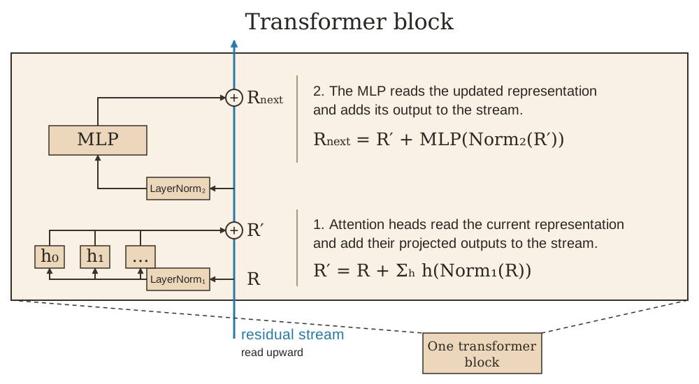
The diagram labels the successive stream states , , and ; these correspond to X, Y, and Z in the code above.
The bypass arrows carry the existing representation. The branches compute updates. This is the residual stream view: successive components read a representation and write contributions back to it. Elhage and colleagues develop that interpretation in A Mathematical Framework for Transformer Circuits; the Transformer interpretability primer, §2 lays out the component equations.
“Partial update” is useful language if it means one component’s contribution to an ongoing representation. It does not imply a small change, a change to only a few coordinates, or an improvement on every step. Updates can reinforce, cancel, or transform what was already there.
For now, assume positional information is supplied. With absolute positions it enters before the first block; other schemes modify attention inside each block. We will return to this distinction after following the two updates.
Exploring self-attention head mechanics
Only a recap is needed here. The head article explains how these operations arise. Let U = layer_norm_1(X) be the normalized read of the stream:
Q, K, V = U @ Wq, U @ Wk, U @ Wv
scores = Q @ K.T / sqrt(d_k)
scores = apply_mask(scores)        # forbidden positions get -inf
A = softmax(scores, axis=-1)
H = A @ V
Q and K are (n, d_k), the mixing weights A are (n, n), and the values and head output are (n, d_v). The head returns mixtures of values, not yet the residual-stream update. In row i, H[i] combines values from all allowed source positions using row i of A.
The matrices Wq, Wk, and Wv are learned parameters shared across positions. Q/K/V and A are computed activations. Deeper in the stack, these projections read representations produced by earlier updates, not fresh lookups of static embeddings. During causal generation, keys and values can be cached; their being computed quantities does not mean they can never be stored.
Multi-head: several mixtures, one attention update
One head provides one distribution over source positions for each receiving position. Several heads can use different distributions and different value transformations at the same time. They need not discover tidy, distinct human-named jobs; the architecture simply gives them that freedom.
Each head receives the full d-dimensional input and projects it to smaller query/key/value spaces. For h heads, a common choice is d_k = d_v = d/h. A head does not receive a raw slice of the input embedding. Efficient implementations project once into a large tensor and then split the projected coordinates into heads.
heads = []
for r in range(h):
    Q = U @ Wq[r]                   # (n, d_k)
    K = U @ Wk[r]                   # (n, d_k)
    V = U @ Wv[r]                   # (n, d_v)
    A = softmax(apply_mask(Q @ K.T / sqrt(d_k)), axis=-1)
    heads.append(A @ V)             # (n, d_v)

delta_attn = concatenate(heads, axis=-1) @ Wo  # (n, d)
Concatenation produces (n, h*d_v). The output projection Wo, shaped (h*d_v, d), maps that result back to the width required by the addition to X.
The output projection turns mixtures into contributions
There is another way to read exactly the same calculation. Split Wo into h row blocks, each of shape (d_v, d). Then:
Each head has a map from its value coordinates into the shared stream coordinates. Project each head’s mixture, then add those contributions. This is algebraically identical to concatenate-then-project, and makes the purpose of W_O concrete. The primer’s §2.1.2 uses this per-head sum form.
The diagram makes those maps explicit for a model with width 768 and 12 heads of value width 64. It follows the contributions into the residual addition at one receiving position. Each head returns a mixture in its own value coordinates, then its output projection expresses that mixture in the shared stream coordinates.
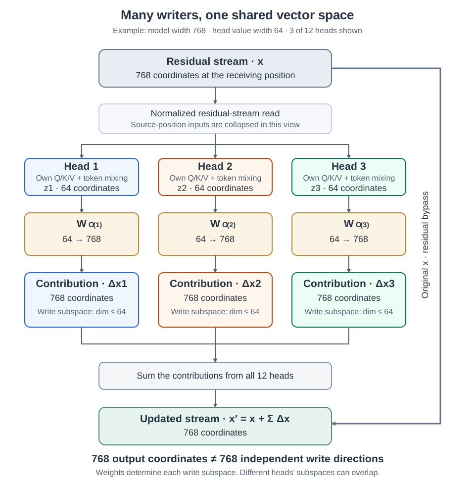
Three of twelve heads are shown; the sum includes all twelve. Each head has its own Q/K/V projections. Splitting the combined output projection into row blocks gives the same result as concatenating the head mixtures and projecting once. This pre-norm view omits source-position inputs, biases, and dropout.
Producing 768 coordinates does not give an individual head 768 independent write directions. With this article’s row-vector convention, each has shape , and its row space is the head’s write subspace, of dimension at most 64. The shared-space article uses the equivalent column-vector convention and explores how these subspaces affect what later components can read.
For one receiving position, a head’s contribution is:
The mixing weights choose how much from each source. The value and output projections determine what vector each source contributes. Holding the weights fixed while changing these projections changes the update. A heatmap therefore cannot tell the whole story of a head’s effect.
A head’s mixture is a convex combination of its value vectors: nonnegative weights summing to one. Applying a linear output projection preserves that property relative to the projected values. But those are not the original input vectors. Summing several heads and adding the result to X does not constrain the updated representation to an average of the original inputs.
Residual connections and layer normalization
We can now incorporate the attention update:
The addition is elementwise and position-preserving. Position i keeps an additive path from its incoming vector and receives the update computed for that position. It does not get replaced by whichever source received the largest attention weight.
A mixture, an update, and an updated representation
Take the head article’s two-dimensional example with its swap-query projection. To isolate addition, omit normalization and use identity output projection just for this arithmetic:
Object at tower | Structure | Paris identity |
|---|---|---|
Incoming representation x | 1.0000 | 0.0000 |
Head mixture h | 0.2483 | 0.5035 |
Projected update h @ Wo, with Wo = I | 0.2483 | 0.5035 |
Result x + h @ Wo | 1.2483 | 0.5035 |
The head mixture alone has less structure content than the input. Adding it gives a representation with an explicit path from the original vector and a new Paris component. This is the distinction between gathering a contribution and updating an existing representation.
Now let the output projection negate the first coordinate: Wo = diag(-1, 1). The update becomes [-0.2483, 0.5035] and the result becomes [0.7517, 0.5035]. The operation is still addition, yet the structure coordinate decreases. An additive path does not guarantee that every feature is preserved: contributions can cancel earlier components.
In the widget, change the query and value transformations, then toggle . Follow the four distinct objects from input to result. It computes the two-dimensional example above, without normalization, to isolate the operations.
Follow the mixture into an update
The receiving position is tower. Its input is [1, 0]. Keys stay unchanged; scores use √2 scaling.
[1.0000, 0.0000][0.2483, 0.5035][0.2483, 0.5035][1.2483, 0.5035]The mixture and update coincide only when Wo is identity. Negating its structure coordinate reduces that part of the result, even though the operation is still addition. This calculator omits normalization to isolate the arithmetic.
Residual learning was introduced in ResNet as learning a correction to an input. Setting a residual branch to zero leaves an identity mapping. In differentiation, y = x + F(x) gives dy/dx = I + dF/dx: the direct path adds an identity term to the Jacobian. This helps optimization, but it is not a guarantee that gradients can never vanish or explode.
Normalize the read, preserve the addition
In our pre-norm baseline, attention receives LayerNorm(X) but its update is added to X, not to that normalized array. The FFN likewise reads LayerNorm(Y) and adds its output to Y. Normalization belongs on the branches; it does not replace the stream at each addition.
The normalization article develops LayerNorm, RMSNorm, and their placement around residual connections. Its key distinction applies here: pre-norm computes x + F(Norm(x)), while post-norm computes Norm(x + F(x)). We use the first arrangement for both attention and the FFN.
Each token is normalized across its own features. The running sum itself is not forced to have unit variance. Pre-norm language models commonly normalize once more before the vocabulary readout.
The original Transformer and BERT use post-norm, so this walkthrough’s pre-norm equations do not describe their exact layout. The Annotated Transformer implementation also notes that its executable code uses pre-norm despite the original paper’s post-norm design. Check placement when comparing diagrams.
The feed-forward sub-layer
Attention has brought information from other positions into Y. Now each position independently computes another contribution:
For our baseline, the FFN is a two-layer MLP:
F = layer_norm_2(Y)                 # (n, d)
hidden = gelu(F @ W1 + b1)          # (n, d_ff)
delta_ffn = hidden @ W2 + b2         # (n, d)
Z = Y + delta_ffn                    # (n, d)
W1 expands the feature width, often to d_ff = 4d, and W2 maps the result back to d so it can be added. The same FFN weights are used at every position. There is no cross-position mixing here: row i is processed using row i alone.
The nonlinearity matters because two consecutive linear maps would collapse into one. With GELU between them, the contribution depends on which intermediate features activate. Attention is already nonlinear through its input-dependent softmax; the FFN adds a different, per-position nonlinear transformation.
The roles are therefore concrete: attention gathers across positions; the FFN transforms within each position; both write updates. The FFN can operate on context because that context has already entered Y. It does not need to look at another row itself.
For a width-768 example, 768 → 3072 → 768 gives the intermediate computation more coordinates, then returns to the stream width. That return is an architectural requirement for the addition, not evidence that all the intervening computation is information-preserving or lossless.
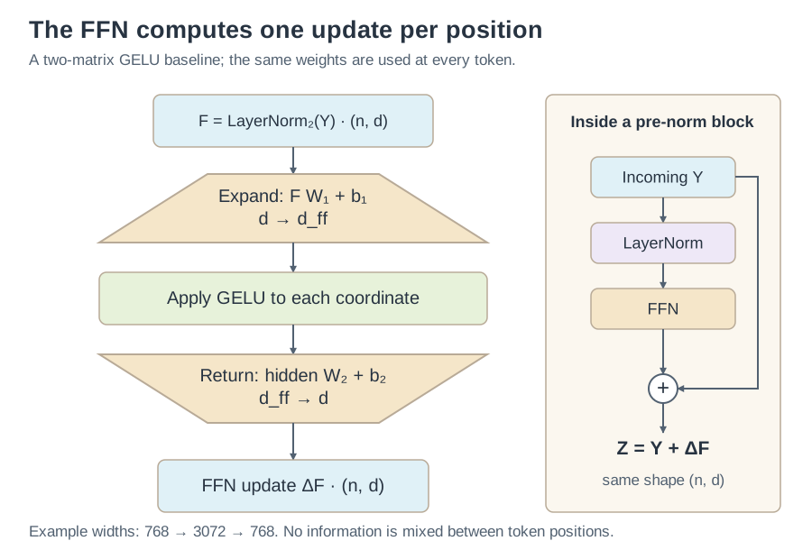
The wide middle is internal to the FFN. Both its input and output have shape (n, d), and each position follows the same computation independently. The inset shows where this update joins the pre-norm residual stream.
Positional encodings: telling the model where each token is
The operations above need information about order. Unmasked self-attention without positional information is permutation-equivariant: permute the input rows and the output rows permute in the same way. The rowwise FFN and normalization do not supply order either. A causal mask does impose an ordering constraint, but it is not interchangeable with a full positional representation.
For absolute positions, the first stream state is:
X = token_embedding(token_ids) + position_embedding(position_ids)
for block in blocks:
    X = block(X)
That positional addition happens once below the stack. It is not the same as the attention and FFN updates inside every block. The position vectors may be fixed sinusoids or learned table entries.
Other schemes introduce position into attention itself:
| Scheme | Where position enters | What the addition/update path sees |
|---|---|---|
| Sinusoidal or learned absolute positions | Added to token embeddings before the first block | A stream initialized with token and position information |
| Relative position bias | Added to query–key scores | Mixtures weighted using content and relative position |
| RoPE | Rotates queries and keys before their dot product | Mixtures whose scores incorporate relative rotations |
With RoPE, keep the underlying query/key content fixed and shift both positions equally: their dot product is unchanged because the relative rotation is unchanged. The score still depends on content, vector magnitudes, and the rotation frequencies; it is not merely a function of distance. The two-dimensional widget isolates the positional effect with unit vectors initially aligned:
Position changes what a head reads or how it matches; it does not replace the value-mixture and residual-addition steps. The modern-model follow-up explores these architectural choices further. Extending a positional formula to larger indices alone does not establish reliable long-context behavior.
Putting the block together
Here is the complete path again. The attention function includes all heads, masking, concatenation, and W_O. Dropout and batch dimensions are omitted:
def block(X):
    U = layer_norm_1(X)
    delta_attn = multi_head_attention(U)
    Y = X + delta_attn

    F = layer_norm_2(Y)
    delta_ffn = gelu(F @ W1 + b1) @ W2 + b2
    Z = Y + delta_ffn
    return Z
Follow the same stages in the explorer. Its dimensions are an illustrative pre-norm configuration (d = 768, 12 heads of width 64, d_ff = 3072), not a claim that this is BERT’s exact norm layout.
The communication step: each token gathers information from the other tokens.
Project into Q/K/V (12 heads × 64 dims each); score every query against every key (Q·Kᵀ / √64), softmax into weights, mix the value vectors by those weights. Concatenate the 12 head outputs and project back to 768 with W_O.
Q: n × 12 × 64
K: n × 12 × 64
V: n × 12 × 64
Attn(X) = Concat(head_1 … head_12) · W_OLearn more: Self-attention mechanics →
Each block has the same input/output shape, so its output can feed the next block. Blocks normally have their own parameters: repeating the architecture does not mean reusing one set of weights. At the next depth, Q/K/V and the FFN read the updated representations, so a later component can respond to information a previous component introduced.
In this pre-norm baseline, expanding the additions gives, before the final norm:
This is a sum of computed, dependent updates. It does not make the network linear: each later contribution depends on the running state produced by earlier ones. The primer’s §2.2 uses this expansion to analyze how components contribute to the final representation. The vocabulary projection reads that final state; it does not write an update back into the block’s stream.
Full attention allows a position to gather from either direction. Causal attention restricts it to itself and earlier positions. An encoder–decoder’s decoder adds a cross-attention sublayer to gather from the encoder’s representations. The architecture article builds these variants from the block, rather than being a prerequisite for this explanation.
Transformer math: sizing a model in your head
The same shapes provide a compact parameter ledger. Assume h*d_k = h*d_v = d, a dense two-matrix FFN with d_ff = 4d, and omit biases and normalization parameters:
| Part of one block | Weight shapes, combined across heads | Parameters |
|---|---|---|
| Query, key, value projections | Three d × d matrices | 3d² |
| Attention output projection | d × d | d² |
| FFN expansion and return | d × 4d, 4d × d | 8d² |
| Total | Six large matrices | 12d² |
An N-block stack therefore has approximately 12 N d² parameters before embedding tables and other small terms. In this baseline, two-thirds of the block’s weights are in the FFN. Gated FFNs, shared key/value projections, and other variants change the arithmetic; the shape method still applies. The GPT-2 walkthrough supplies a concrete model-wide count.
Sequence length changes activation and compute costs, not these projection matrix sizes. Full-sequence attention’s score and value-mixing work scales as n²d; projection and FFN work scales linearly with n for fixed width. Efficient attention kernels can avoid storing the entire score matrix, but that does not remove the pairwise arithmetic. Cached single-token decoding has a different cost profile: its new query reads the existing keys and values.
There is no universal context ceiling at 200K tokens. Model design, memory, kernels, positional training, batch size, and acceptable latency all matter. The KV-cache article derives the memory bill; inference optimization follows the serving consequences.
From one contribution to a stack
A head computes a mixture. The output projection expresses it as a contribution in stream coordinates. Attention’s contribution is added to the representation, then the FFN computes and adds another. Stacking repeats that sequence on increasingly transformed inputs.
That is the connection between the toy and the block: mixing determines what information arrives; additive updates determine how each component joins the running representation. The shape stays (n, d) while the information in its rows changes.
To see a full model execute, use Brendan Bycroft’s visualizer and follow one residual path alongside its branches. Then continue to encoders, decoders, and the architectural split, or the GPT-2 pipeline.
Optional: how much of this picture is real?
Geometric examples, head roles, and what an attention map can establish
The operations are literal; the labelled axes and narrative roles in our toy are chosen for teaching. Real learned features need not occupy individual coordinates. A head may participate in multiple behaviors, and several heads may contribute to the same behavior. Parallel heads in a layer and successive layers are different forms of composition; neither guarantees a clean progression from syntax to semantics in every model.
An attention map is a measurement of A. Its value for explaining behavior depends on the values being mixed, output projections, other components, and what the downstream computation reads. The head article’s real-model exercise distinguishes inspecting weights from testing a proposed mechanism. Do not infer a unique semantic role from one attractive heatmap.
The residual stream has finite width. Adding contributions in shared coordinates does not create separate permanent storage slots for each head or layer. Directions may overlap, reinforce, or cancel. The sparse-autoencoder article explores why individual coordinates can be difficult to interpret.
Alternative norms, gated FFNs, and learned factual associations
RMSNorm rescales a row without subtracting its mean. Some architectures normalize at additional points, use gated feed-forward networks such as SwiGLU, or omit selected biases. These change the branch computations and sometimes their arrangement; inspect the specific model rather than treating one diagram as universal. The modern-LLM article compares such choices.
Interpretability work also studies FFNs as learned memories. ROME investigates factual associations and targeted weight edits in particular transformer MLPs. This does not mean every fact occupies one neuron or only FFNs store knowledge. It is a research direction to explore after the forward computation is clear.
Further connections and companion readings
The head article’s mathematical notes retain the bilinear-score, kernel, and fast-weight-memory connections. Linear attention changes the mixing rule; it is not just another placement of the residual addition.
For implementations, the Annotated Transformer pairs code with the original paper; check its explicitly noted pre-norm code choice. Inside the Transformer: The Life of a Token is a complementary walkthrough with concrete tensor shapes and architectural variations. The interpretability primer goes beyond following the computation to methods for investigating what trained components do.