Recovering known features with two attention projections
Can a tiny attention model learn to read identifiable features from mixed input coordinates? We can test this without training a language model: construct data whose features we know, hide those features through a linear mixing operation, and train only a query projection and a value projection.
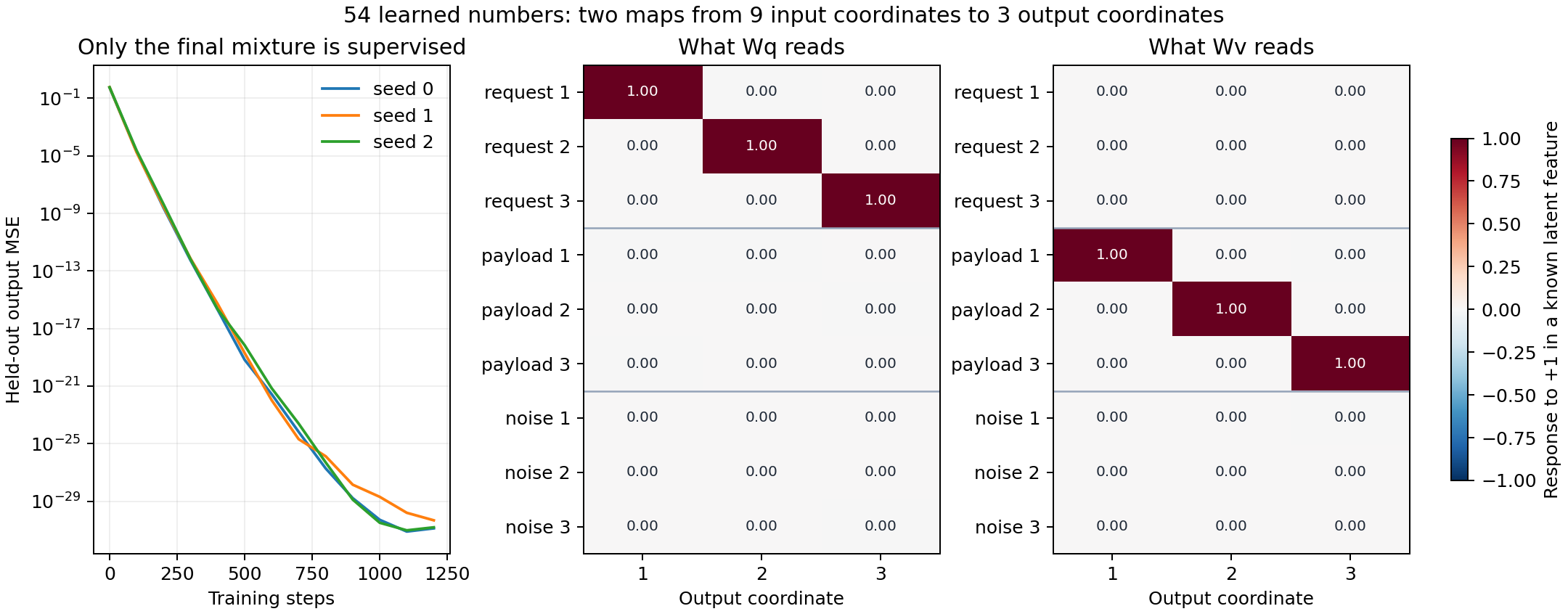
This experiment has 54 trainable numbers: two 9 × 3 matrices, Wq and Wv. Each query and value has three coordinates. Across three initializations, the model recovered the intended feature responses to floating-point precision on fresh evaluation examples. Removing relevant features increased prediction error, while changing irrelevant inputs barely affected the output.
The result is deliberately controlled. Fixed keys and direct output targets anchor the feature meanings so we can identify them. It demonstrates recovery of known synthetic features through an attention loss; it does not establish that a freely trained language model will develop equally readable coordinates.
The attention-head article introduces queries, keys, and values. Here we use that computation as a small experimental system.
The task: route a request and return three values
Each example contains one request and four source records. Before hiding the features, each input has nine independent scalar coordinates:
| Latent coordinates | Role in the task |
|---|---|
| Request features 1–3 | Control routing when this input is the request |
| Payload features 1–3 | Supply the values to return when this input is a source record |
| Noise features 1–3 | Irrelevant to the target |
These labels describe how the data generator uses the numbers. They are not natural-language concepts. In the request input, the payload coordinates are also irrelevant; in the source records, the request coordinates are irrelevant to the value calculation.
We draw the latent coordinates from independent normal distributions, scaling the request’s first three coordinates by 1.8 to vary attention concentration. A fixed random orthogonal matrix R mixes every input:
The model sees the nine observed coordinates of x. It receives neither the original feature vector z nor the mixing matrix R. The useful features are distributed across the observed coordinates rather than occupying designated input slots.
The data generator also supplies four fixed keys:
fixed_keys = torch.tensor([
    [ 1.,  1.,  1.],
    [ 1., -1., -1.],
    [-1.,  1., -1.],
    [-1., -1.,  1.],
])
To generate the correct target, the teacher uses the request’s three original request features as a query, compares it with those keys using scaled dot products and softmax, and takes the corresponding weighted average of the records’ three payload features. The target is therefore a three-coordinate vector.
The student receives only the final target, not the teacher’s intermediate query, values, or attention weights. The teacher’s construction gives us known ground truth for evaluation.
The model: two learned matrices
The model follows the same attention computation, but it must learn how to extract useful features from the mixed inputs:
q = request @ Wq                          # (batch, 9) → (batch, 3)
V = records @ Wv                          # (batch, 4, 9) → (batch, 4, 3)
A = torch.softmax(q @ fixed_keys.T / 3**0.5, dim=-1)
prediction = (A.unsqueeze(-1) * V).sum(dim=1)
loss = ((prediction - target) ** 2).mean()
Only Wq and Wv are trainable: 9×3 + 9×3 = 54 scalars. There is no learned embedding table, key projection, output projection, bias, classifier, feed-forward network, or residual block. This is a restricted fixed-key attention task, with one receiving request and four source records.
The query map must learn the request features that determine routing. The value map must learn the payload features that determine what gets returned. Both are optimized jointly using the final prediction error. Backpropagation must find useful query and value representations without direct labels for those representations.
What does the value part contribute?
The complete computation has two parts:
The query and keys determine how much to take from each record. The values determine what information those records contribute. Here A is a row of four weights, V contains four three-coordinate value vectors, and their product is the three-coordinate prediction. Computing A alone gives a distribution over records; multiplying by V gathers their information into the output.
For a small arithmetic illustration, suppose the weights and values are:
| Record | Attention weight | Value vector | Weighted contribution |
|---|---|---|---|
| 1 | 0.1 | [1, 0, 0] | [0.1, 0, 0] |
| 2 | 0.2 | [0, 2, 0] | [0, 0.4, 0] |
| 3 | 0.3 | [0, 0, 3] | [0, 0, 0.9] |
| 4 | 0.4 | [1, 1, 1] | [0.4, 0.4, 0.4] |
Adding the contributions gives . These are illustrative numbers, rather than a recorded evaluation example.
Now hold the query and keys fixed and swap the first two output columns of Wv. Every value vector swaps its first two coordinates, so the output becomes . The attention weights stay exactly the same. The model gathers from the same records in the same proportions, but returns different information. The value-swap widget in the attention-head article demonstrates this distinction interactively.
In our experiment, Wv must learn to extract the three payload features from each record’s nine mixed coordinates and ignore the request and noise features. It is one shared learned matrix applied to all four records, producing four computed value vectors on each pass. The payload vectors are not separate trainable entries. The final prediction loss teaches Wv what to pass on, while also teaching Wq how to weight the records. Because this experiment has no output projection, the weighted value mixture is already the prediction; in a full transformer block, an output projection and residual addition incorporate the head mixtures into the running representation.
Why fix the keys?
In a freely trained head, a change of query basis can be compensated by an inverse change of key basis. The attention scores remain the same, so the query coordinates alone are not uniquely determined. Our attention-head mathematics section explains this ambiguity.
Fixing the keys anchors the query matching coordinates. The four keys above are tetrahedron vertices whose differences span all three matching directions. We use four keys because softmax is insensitive to adding the same constant to every score: three keys could constrain at most two independent score differences, leaving a query direction unidentifiable in a three-dimensional query space.
The direct three-coordinate target similarly anchors the value output meanings. We have deliberately made the representations easier to identify than those of a general transformer. That is useful for this experiment: it lets us test whether optimization recovers known features before tackling representations with arbitrary internal bases.
Measure what the learned maps read
We know the latent-to-observed mixing matrix, so we can inspect the learned maps in the original feature basis:
Each entry of R @ Wq measures how increasing one latent feature by one changes one query coordinate. Likewise, R @ Wv measures the response of a value coordinate. This is a direct measurement of the learned linear maps, without fitting an additional probe that could rotate or remix their outputs.
The expected query response reads the first three latent features and ignores the other six. The expected value response reads the middle three features and ignores the remaining six. In terms of subspaces, the maps should read different three-dimensional input subspaces and ignore their respective perpendicular complements.
Results on held-out examples
The checked runs used PyTorch 2.7.1+cpu, float64 arithmetic, one CPU thread, Adam with learning rate 0.03, and 1,200 steps. Each step used a fresh batch of 128 training examples. Each run also had 4,096 separate evaluation examples; evaluation did not control optimization or early stopping.
| Seed | Held-out prediction MSE | Uniform attention with true values: MSE | Smallest query/value coordinate R² |
|---|---|---|---|
| 0 | 1.30e-31 | 0.332 | above 0.999999 |
| 1 | 4.70e-31 | 0.332 | above 0.999999 |
| 2 | 1.53e-31 | 0.334 | above 0.999999 |
The model recovered the expected feature responses to floating-point precision. The uniform-attention comparison uses the true payload values, giving that baseline the correct content but no request-dependent routing. Its much higher error shows why a plain average does not solve this task.
These are noiseless targets generated by a computation the student can represent exactly. The very small error demonstrates successful recovery in this construction, rather than a realistic accuracy expectation for natural data.
Do the recovered features affect the prediction?
A response heatmap shows what a linear map reads. We also test how those inputs affect the final prediction by intervening on known latent coordinates and then applying the same fixed mixing matrix.
| Intervention | Measurement across the three seeds |
|---|---|
| Erase one request feature, keeping the original target fixed | Prediction MSE rises to 0.139–0.153 |
| Erase one payload feature from every source record, keeping the original target fixed | Prediction MSE rises to 0.188–0.207 |
| Add 5 to every coordinate irrelevant to each map | Prediction change is about 1e-30 to 7e-30 in MSE |
The first two interventions remove information the task uses; the ranges cover all three feature choices and all three seeds. The last changes irrelevant inputs: the request’s payload and noise coordinates, and the source records’ request and noise coordinates. The prediction remains effectively unchanged.
Together, the learned-map responses, held-out predictions, and interventions support a precise conclusion: these two learned matrices recover and use different known feature sets while ignoring irrelevant input directions on this task.
Reproduce the experiment
From the repository root, with PyTorch and Matplotlib installed:
python blog/src/content/drafts/recovering-known-features-with-two-attention-projections/experiment/train_feature_recovery.py
python -m unittest discover -s blog/src/content/drafts/recovering-known-features-with-two-attention-projections/experiment -p 'test_feature_recovery.py' -v
The script writes feature-recovery/results.json, containing the fixed keys, input mixing matrix, raw learned projections, measured feature responses, loss traces, held-out metrics, and intervention results. It also generates the PNG and SVG figure. The tests check that only the two intended matrices are trainable, that the known solution reproduces the teacher after mixing, and that the key differences span all three query directions.
The experiment makes the meanings testable through its construction. For a head learned from text, we would need independent evidence to identify useful feature directions, account for changes of basis, and test their effects. The attention-head article returns to the more general computation: match with queries and keys, then mix the information carried by values.