Feature detectors: how neurons read and write
Neural networks learn to recognize patterns and use them to make predictions. How those patterns are represented inside a network remains an open research question. Distill’s work on understanding neural networks proposes that features are the fundamental units of neural networks. This makes it interesting to explore how a neural network can implement a feature detection mechanism.
To understand this mechanism, we will begin with a single neuron. Its incoming weights determine which parts of the input to emphasize, suppress, or ignore, allowing it to act as a feature detector that responds to a particular pattern. Our exploration will be based on a small spam classifier, where a neuron’s response to a combination of promotional words helps the output neuron decide whether the message is spam.
Then we will bring several of these feature detectors together in a layer, each using different weights to respond to a different pattern in the same input. In our spam classifier, one neuron responds to promotional words while another responds to words common in routine messages. Their responses give the next layer several signals to combine, allowing the prediction to depend on multiple patterns rather than a single detector.
We choose the detector roles and weights by hand to make the calculations easy to follow and each neuron’s contribution easy to inspect. In a trained network, those roles emerge as learning adjusts the weights, and individual neurons can develop overlapping responses that do not fit such clear categories. Our example gives us a simple setting in which to understand the mechanism before examining what training produces.
Dimensions count coordinates
Let’s first look at how a message becomes a point in a feature space. We will choose a few words and count how many times each appears in the message, then use those counts to calculate a spam or non-spam prediction. We choose the vocabulary and weights by hand so that each calculation can be followed. A training demonstration later uses the same encoding with learned weights.
First, we need to define our vocabulary: the words we will track, arranged in a fixed order. Every message will use the same list: one count per vocabulary word, with zero for an absent word. Words outside the vocabulary are ignored. To see how this works, we will start with just two words: claim and prize.
The table shows a small illustrative dataset, with each message’s label and its counts for our two vocabulary words. We treat uppercase and lowercase letters alike and ignore punctuation:
| Message | Claim | Prize | Label |
|---|---|---|---|
| Claim your prize. Claim it at the meeting. | 2 | 1 | Spam |
| The project meeting is tomorrow. | 0 | 0 | Non-spam |
| Prize! | 0 | 1 | Spam |
We can now combine the first message’s counts into a vector , where the first entry is the claim count and the second is the prize count. These two numbers are the vector’s components, also called its coordinates. The number of coordinates defines the vector’s dimensionality, so our vector is two-dimensional. This is word-count encoding, a bag-of-words representation: it records how often words occur but discards their order in the message.
You may have seen a vector like this defined in PyTorch:
import torch

x = torch.tensor([2, 1])
Its shape is (2,): one array axis containing two entries. PyTorch calls this a one-dimensional tensor, because x.ndim counts array axes. In our geometric description, it represents a two-dimensional vector, because it has two coordinates.
This two-dimensional vector can be plotted on a plane with the horizontal -axis marking the claim count and the vertical -axis marking the prize count. The message sits at the point : 2 along the claim axis and 1 along the prize axis.
If we want to start tracking another word, such as meeting, we add its count as a third coordinate, giving our vector another dimension. Here is the extended table:
| Message | Claim | Prize | Meeting | Label |
|---|---|---|---|---|
| Claim your prize. Claim it at the meeting. | 2 | 1 | 1 | Spam |
| The project meeting is tomorrow. | 0 | 0 | 1 | Non-spam |
| Prize! | 0 | 1 | 0 | Spam |
In the first message, meeting appears once, so the vector becomes . All three coordinates are nonzero. Other messages still record zero for absent words. The coordinate order is claim, prize, then meeting.
Each word count is an input feature and occupies one coordinate, corresponding to an axis in feature space. Moving along the axis for the claim count changes that count while leaving the others fixed. These counts are discrete: a word can appear once or twice, but not 1.5 times.
Here, the input features have clear meanings because we chose the encoding: one coordinate per word in our vocabulary. We will also choose the detector weights by hand so we can follow how they combine these counts. However, in many text models, a tokenizer instead converts each message into a sequence of token IDs, representing words or parts of words. The model maps these IDs to learned vectors called embeddings. Training adjusts the embeddings and the network’s weights so it can learn useful patterns without us assigning particular word groups to individual neurons.
We assign an axis to each input feature. Since the count of each word we track is one feature, the vocabulary size determines the input vector’s dimensionality. With a vocabulary of 100 words, every message gets 100 coordinates, whether it contains 3 words or 300. A message can be any length: additional words may change the counts, but they do not add coordinates. We cannot draw all 100 axes together, but we can still store the values and calculate with them.
Our complete vocabulary is ['claim', 'prize', 'meeting']. Every message gets three coordinates, including zeros for absent words:
| Message | Word-count vector |
|---|---|
| Prize! | |
| Claim your prize. Claim it at the meeting. | |
| The project meeting is tomorrow. | |
| Claim your prize at the meeting. |
A vector with mostly zero entries is called sparse. “Prize!” has two zero entries out of three. With a larger vocabulary, a short message might use only a small fraction of the available words; the rest would still receive zero counts.
One neuron combines three inputs into one score
We now encode a message as three features: the counts of claim, prize, and meeting. Now let’s see how a neuron can use these features to detect a pattern. The neuron stores one weight for each input coordinate, determining how much that input contributes to the result. It then multiplies each input coordinate by its corresponding weight and adds the contributions to produce a single response score. Training adjusts these weights to change how the neuron responds to its inputs.
This calculation is a weighted sum:
Here is the value of input feature , and is its corresponding weight. The inputs form the vector , and the stored weights form the neuron’s incoming weight vector . We can also name a coordinate by its feature: denotes the claim count in the input vector .
The full neuron calculation then adds a bias to this score and applies an activation function , which can introduce nonlinearity. This produces the neuron’s output :
To make the demonstration simpler, we will use zero bias and an identity activation function, so the output is the weighted sum itself:
The diagram below shows this calculation for our message vector : each count is multiplied by its corresponding weight, and the three contributions are added to produce the score .
Notice what this mechanism allows the neuron to do: by setting some weights to zero, it can ignore those input coordinates and respond only to the others. A count multiplied by zero contributes nothing to the sum; a negative weight makes a positive count lower the score.
For example, to make the neuron respond only to the claim count, give claim a weight of 1 and every other word a weight of 0. Its stored weight vector is therefore . When the neuron processes our input, it computes the weighted sum:
Our input vector now has three nonzero entries, while the chosen weight vector has two zeros. A zero means different things in these two kinds of vectors: a zero input count means the word is absent, while a zero weight means the neuron ignores that word, even when it is present. Vectors with many zero entries are called sparse; our chosen weight vector has two zeros out of three entries.
So far, our neuron has used only one input feature: the claim count. But it can also combine several features by giving them nonzero weights. For example, we can create a promotional reader that responds to claim and prize while ignoring meeting. Let’s give claim a weight of and prize a weight of , while keeping meeting at :
When the neuron computes the weighted sum for the same message using these new weights, we get:
With these weights, each occurrence of claim contributes to the score, each prize contributes , and meeting contributes nothing.
This detector responds to claim and prize regardless of their meaning in context: “prize” could also appear in a legitimate announcement. For a trained neuron, we must examine its responses to many inputs before assigning it a label such as “promotion detector.”
It’s also possible to make a feature suppress the neuron’s response by giving it a negative weight. For example, computes the prize count minus the meeting count: each occurrence of meeting lowers the score by . Equal counts cancel, so a zero score does not necessarily mean that the input is zero.
The weights define a reading direction
Let’s now introduce a little linear algebra and see how the input and weight vectors relate geometrically. We already plotted the vector for one of our example messages in a three-dimensional space with claim, prize, and meeting axes. We can now plot the neuron’s weight vector in that same space and compare their directions.
The weight vector defines the neuron’s reading direction: its relative weights determine which combination of input coordinates it measures. The dot product measures how much of the input lies along this direction, scaled by the weight vector’s length. We can calculate it using the vectors’ coordinates:
As you can see, it’s the same arithmetic as the weighted sum we saw earlier. Scalar algebra expresses it as a weighted sum, while linear algebra expresses it as a dot product between vectors. In the formula above, we write and as column vectors with three rows and one column, and use to represent the weights as a one-row, three-column matrix so that multiplying it by the input column produces one score.
For nonzero vectors, we can also express this same dot product geometrically, using the vectors’ lengths and the angle between them:
where is the angle between the input and the reading direction. With both lengths fixed, an input pointing closer to the reading direction produces a larger score. An input perpendicular to it produces zero.
The formula above has two parts: the length product , which sets the scale, and , which captures the vectors’ alignment. For example, doubling the weights to preserves the reading direction but doubles every score. The dot product therefore reflects both the vectors’ alignment and their lengths.
Let’s now explore this relationship in the widget below. The promotional reader’s weight vector is shown in blue and the message vector in orange. Their dot product is the score we calculated above. All three input coordinates are visible, so the plot shows the full input and reading direction.
Drag the plot to inspect the two arrows. reveals how the weight coordinates build the blue arrow; adds the geometric measurements.
The promotional reading direction
Reader w = (1.5, 1, 0)
Input x = (2, 1, 1)
The component arrows describe the weights themselves, not the products of weights and input counts. The green projection shows the part of the input along the reader. Since the reader’s meeting weight is zero, adding meeting counts moves the input perpendicular to the reading direction and leaves its score unchanged, regardless of how many times meeting occurs.
From feature detectors to a layer
By giving claim and prize nonzero weights and meeting a zero weight, we made the neuron respond to a combination of claim and prize counts while ignoring meeting. This is how our neuron acts as a feature detector: its score measures a particular combination of input features. We use to denote a neuron’s weighted-sum score and add a subscript to identify the detector. So, for the promotional detector, the formula is:
Each additional occurrence of claim raises the score by , and each additional prize raises it by . Adding meeting leaves the score unchanged because its weight is zero.
A message can contain many different patterns, and different neurons can respond to different combinations of its features. To detect another pattern, we can introduce a second neuron that receives the same three word counts. Let’s use the word “meeting” for a routine-message pattern, giving it a weight of and setting the claim and prize weights to :
Let’s apply these weights to our starting message and to the project-meeting message:
| Message | Score | |
|---|---|---|
| Claim your prize. Claim it at the meeting. | 2 | |
| The project meeting is tomorrow. | 2 |
We now have two neurons receiving the same three-coordinate input . Each produces one scalar response, and these responses together form the layer’s output vector :
| Message | Promotional response | Routine response | Layer output |
|---|---|---|---|
| Claim your prize. Claim it at the meeting. | 4 | 2 | |
| The project meeting is tomorrow. | 0 | 2 | |
| Prize! | 1 | 0 | |
| Claim your prize at the meeting. | 2.5 | 2 |
The diagram below shows how both neurons receive the same three word counts and use their own weights to produce the two coordinates of .
We can describe the layer shown above in matrix form by collecting the neurons’ weight vectors into one weight matrix . The first row contains the promotional neuron’s weights, and the second contains the routine neuron’s weights:
Each row corresponds to one neuron, and each column corresponds to one input feature: claim, prize, or meeting. This makes a matrix. Multiplying it by the three-coordinate input vector computes both neurons’ weighted sums at once:
The result is the layer’s activation vector, with one coordinate per neuron’s output after its activation function. The matrix–vector multiplication above is the same calculation shown in the diagram. Because we don’t use biases or nonlinear activation functions in this example, the weighted sums pass through unchanged, so is both the pre-activation vector and the activation vector.
When a neuron has a large positive activation, we informally say it is firing strongly. We call an activation large relative to that neuron’s usual responses across inputs; other neurons may operate on different scales. The underlying dot-product score depends on the input and weight vectors’ lengths and their alignment. Bias and the activation function can then modify this score to produce the neuron’s output.
Our two neurons illustrate specialization: one responds to promotional words and the other to routine-message words. Both receive the same input vector but store their own weights. We deliberately set a weight to zero for each input feature we want a neuron to ignore. In trained networks, these weights are usually nonzero, so neurons typically combine many of the same input features, giving each a different influence through their learned weights.
One output neuron combines the responses into a prediction
Our first layer produces the activation vector , containing the promotional response and routine response . To use these detected patterns to decide whether the message is spam or non-spam, we’ll add a classification neuron that takes these responses as inputs and combines them into a single score. It uses the same weighted-sum mechanism, but now combines detected patterns rather than individual word counts.
Because we have only two classes—spam and non-spam—this is a binary classification problem. We can use a single classification score and choose the class from its sign: positive means spam, negative means non-spam, and zero marks the decision boundary, where our manual rule gives neither class a preference.
We want a stronger promotional response to move the prediction toward spam and a stronger routine response to move it toward non-spam. To achieve this, we’ll set the classification neuron’s weights to for the promotional response and for the routine response, keeping its bias at zero. The classification score is described by the formula , where denotes the classification score.
Use the controls below to change the promotional and routine responses and see how their weighted contributions move the classification score along the number line.
We chose the classification neuron’s weights, and , to make the calculation easy to follow. They are not necessarily optimal for real messages; training can learn these weights along with the feature detectors’ incoming weights.
Just as we collected the feature detectors’ weights into matrix , we can collect the classification neuron’s weights into matrix . This weight matrix has one row and two columns. We write the hidden layer’s output as a column vector, with the promotional response followed by the routine response , so that multiplying by gives the classification score :
Whether chosen by hand or learned through training, these weights produce a classification score that can be negative or greater than . A probability, however, must lie between and . To express the result as a probability, we could apply the sigmoid function to the completed score:
A positive score gives a probability above ; a negative score gives one below . Thresholding that probability at is equivalent to checking the score’s sign. This conversion does not change the decision, and hand-chosen weights do not guarantee calibrated probabilities.
Sigmoid converts one score into one probability; here, the probability of non-spam is . If the output layer instead produced several scores, one for each mutually exclusive class, we would use softmax to convert them together into class probabilities that sum to .
With the classification neuron in place, we now have a complete network. The diagram below shows three input units, one for each word count; two hidden neurons, which detect promotional and routine-message patterns; and one output neuron, which combines their responses into a classification score.
We can now follow a message through the whole network: from three word counts to two detector responses, which are then combined into one classification score. Use , , and to view one stage at a time: the input in 3D, the hidden responses in 2D, and the final score on a number line. The word counts stay the same when you switch views.
Starting with “Claim your prize. Claim it at the meeting.”, change from 1 to 2. The input moves along the meeting axis, and the routine response rises from 2 to 4 while the promotional response stays at 4. The hidden point reaches the decision boundary , and the classification score falls from 2 to 0. Increase the meeting count further to move into the non-spam region, where the final score is negative.
1. Input space: two detectors read x
x = (2, 1, 1)
Green w₁ = (1.5, 1, 0) · Angle to x: 25.1° · dot product: 4
Purple w₂ = (0, 0, 2) · Angle to x: 65.9° · dot product: 2
From activations to vector contributions
We have seen how the classification neuron reads the two detector responses. We can also follow what each detector contributes to that neuron. This is the writing view: the detector’s activation scales its outgoing weight to produce a contribution to the next layer.
Keep three quantities separate. For the routine detector, is its activation, is its outgoing weight, and is its contribution to the classifier’s score. The activation measures the detected pattern; the outgoing weight determines how that response affects the receiving neuron.
Our classifier has only one receiving neuron, so each detector contributes one number. If the next layer had several neurons, each detector would have one outgoing weight for each of them. Together, those weights form its outgoing weight vector . The same scalar activation scales every entry:
This vector is column of the next layer’s matrix : its entries connect source neuron to each receiving neuron. For our classifier, the columns are the one-coordinate vectors and . With several receiving neurons, each column would have several coordinates, and each detector would contribute a vector in that larger output space.
The outgoing vector sets the writing direction. A positive activation scales the contribution along that direction, zero contributes nothing, and a negative activation reverses it. During a forward pass, the outgoing weights stay fixed while the activations depend on the input.
For the whole layer, the contributions add together with the next layer’s bias:
Here is the next layer’s pre-activation vector; its activation function is applied afterward. The same activation is therefore both a detector’s response to its input and the scaling coefficient for its contribution to the next layer.
Choosing a reading or writing view
Both views follow the same connections in :
| Perspective | What we follow | What it explains |
|---|---|---|
| Receiving neuron as a reader | One row of | Which combination of incoming activations makes that neuron respond. |
| Source neuron as a writer | One column of | How that neuron’s activation contributes to each receiving neuron. |
This column view also applies to the first layer: each word count scales a column of , and those contributions add to form the two detector responses. The optional layer transformation section works through that calculation.
For more on the space spanned by these outgoing vectors, see vector decomposition and subspaces.
Why two linear layers still give one linear transformation
In our original classifier, we explored reading and writing without introducing any nonlinearity between the layers: each hidden neuron passes its weighted sum directly to the output neuron. This made the mechanism easy to follow, but it also limits what the network can express. To model relationships beyond a single weighted sum of the original inputs, we need a nonlinear activation between the layers. Without one, adding linear layers still gives a single linear transformation.
To see why, recall that with our identity hidden activations and zero biases, the hidden activation vector is and the classification score is . Substituting the first expression into the second gives
The column view explains why this works. Each column of describes how one word count contributes to the hidden activation vector. Multiplying by transforms each of those columns into its contribution to the final score:
| Input coordinate | Column of | After applying |
|---|---|---|
| claim | ||
| prize | ||
| meeting |
These transformed columns form the product :
Because is linear, combining the columns of and then transforming the result gives the same answer as transforming each column first and then combining them. The word counts supply the same scaling coefficients in either calculation. The product therefore takes the original input directly to the score.
So the same score can be calculated directly from the word counts:
One output neuron with those three incoming weights would produce exactly the same score for every input. Our hidden layer gives us an interpretable intermediate representation, but stacking linear layers does not expand the kinds of input-to-score functions we can represent. Applying sigmoid afterward gives the same probability in either arrangement.
To make the hidden layer express a nonlinear relationship, we can apply a nonlinear activation to its weighted sums before the output layer combines them. We will use ReLU: it lets a detector contribute only when its weighted sum crosses a threshold set by its bias. A bias alone would only shift a linear transformation; the nonlinear activation is what generally prevents the two layers from collapsing into one fixed affine transformation.
Adding nonlinearity with ReLU
We can now add the nonlinear step our original classifier was missing. Each hidden neuron still reads the input with a dot product, but we add a bias and apply ReLU before passing its response to the output layer. The bias sets the threshold; ReLU makes responses below that threshold zero. Let be the dot-product score, the score after adding a bias , and the activation passed to the next layer:
ReLU passes positive pre-activations through and replaces negative ones with zero. Add bias to the promotional reader:
Our original message has raw score , so its pre-activation and activation are . A message containing claim once and none of the other selected words has raw score , pre-activation , and activation . This reader now contributes only when its weighted count exceeds . Repetition alone can cross that threshold; both promotional words need not appear.
This changes how additional evidence affects the response. Increasing the raw score from to leaves the activation at , while increasing it from to raises the activation from to . The same increase has a different effect depending on whether the detector is above its threshold. One fixed weighted sum cannot reproduce both behaviors across inputs.
Keeping the routine bias at zero and the outgoing weights unchanged, the original message now gives and , predicting non-spam. We changed the model by adding the promotional bias and ReLU. The earlier widgets continue to show the original manual model.
The activation acts on the total after the bias. It does not filter terms inside the dot product separately: with zero bias, contributions and give , whereas clipping each contribution first would give . Cancellation happens before the activation sees the score.
A detector’s own response can be negative if its activation function permits it. For example, weights applied to our original input give raw score . A bias can also turn a positive raw score into a negative pre-activation. Identity activation preserves that negative value, ReLU replaces it with zero, and activations such as tanh can produce negative outputs.
A nonnegative activation can still lower the next neuron’s score through a negative outgoing weight. Our routine detector does this with , even when it uses ReLU. Conversely, a negative activation paired with a positive outgoing weight also lowers the receiving neuron’s weighted sum: the contribution’s sign depends on both factors in .
With bias and nonlinear activation included, the whole network now computes
Here acts on each hidden pre-activation, and is the output neuron’s scalar bias. Incoming rows still read the input, hidden neurons still supply scalar coordinates, and those scalars still multiply outgoing columns. Bias and activation change how we obtain the scalars. Unlike the identity-activation case, a network with ReLU generally cannot be replaced by one fixed matrix across all inputs.
Training the classifier on real messages
So far, we have chosen the weights and biases ourselves. We now train the same three-input, two-hidden-neuron, one-output architecture on real labeled SMS messages. The hidden neurons use ReLU, and training starts from fresh random weights rather than assigned promotional and routine roles.
We use the SMS Spam Collection, remove duplicate messages after normalizing case and whitespace, and reserve 20% of each class for testing. This leaves 4,128 training messages and 1,031 held-out messages. Each input still contains only the counts of claim, prize, and meeting. The spam/non-spam labels come from the dataset; held-out messages are not used to update the weights.
In our recorded CPU run with PyTorch 2.14.1, seed 42, and 40 epochs, training loss decreased from 0.614 to 0.326. On 1,031 held-out messages, accuracy was 90.0%, compared with 87.6% for always predicting non-spam. Spam recall was 19.5%: the model detected 25 of 128 spam messages. 996 held-out messages had the same all-zero input vector. No choice of weights can distinguish those messages using this encoding alone. The saved run report records the settings, dataset checksum, split sizes, and results.
What did the trained neurons actually learn?
We can test the reading-and-writing explanation against the trained model. We reproduced the saved run exactly, including its weights and training losses, then recorded both neurons’ responses on every held-out message. We also disabled individual neurons and changed word counts to see how those interventions affected the score. These calculations inspect the model directly: each neuron’s contribution is its activation multiplied by its outgoing weight.
The learned parameters are shown below, rounded to four decimal places. Here we use the code’s zero-based names, neuron 0 and neuron 1, without assigning their roles in advance.
| Parameter | Neuron 0 | Neuron 1 |
|---|---|---|
| Incoming weight for claim | +2.5743 | −1.2761 |
| Incoming weight for prize | +2.5039 | −1.3264 |
| Incoming weight for meeting | −0.1353 | +2.6763 |
| Hidden bias | −0.0160 | +1.2650 |
| Outgoing weight into the spam score | +3.0799 | −1.5553 |
The output bias is −0.1484. Neuron 0 resembles our promotional reader: claim and prize increase its response, and its positive outgoing weight turns that response into positive spam evidence. Meeting slightly suppresses it. Both learned readers use all three coordinates, unlike the disjoint groups in our hand-chosen example.
Neuron 1 does more than detect meeting. Its positive bias makes it active even when all counts are zero. At that input, its activation is 1.2650, and its negative outgoing weight produces a contribution of −1.9674. Including the output bias gives a score of −2.1158. It supplies default non-spam evidence; meeting strengthens that evidence, while claim and prize reduce its activation. The activation itself remains nonnegative—the negative contribution comes from the outgoing weight.
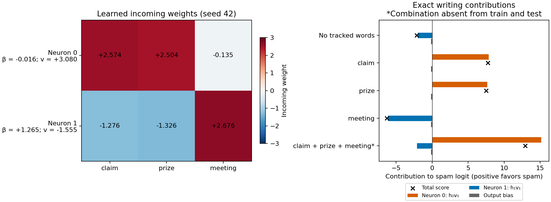
These responses also occur on real messages. One held-out spam message has counts and gives a learned score of 23.3715. That exact count vector is absent from training. A held-out non-spam message, “Sorry, I’ll call later in meeting.”, has counts : neuron 0 is off, neuron 1 contributes −6.1300, and the final score is −6.2783.
For the input , the full contribution breakdown is:
| Part of the learned calculation | Contribution to the score |
|---|---|
| Neuron 0, activation | |
| Neuron 1, activation | |
| Output bias | |
| Final score, computed before rounding |
The score is positive, so this message is predicted as spam. These values come from the recorded run and are rounded for display. The two contributions plus the bias reproduce the normal forward pass, even though training can change the detectors’ roles.
The interpretation has limits. Neuron 1 also activates on all 103 spam messages the model misses. Calling its contribution “non-spam evidence” describes how the model uses it, not a guarantee that the message is legitimate. No message in either split combines meeting with claim or prize, so the mixed example in the figure is a synthetic probe of the model. Our hand-written input is also an illustrative mixed input, not a recorded dataset example.
Disable a neuron and measure its effect
To test each neuron’s role, we set its activation to zero on every held-out input, keeping the other activation, weights, and biases fixed. This removes exactly its contribution; we do not retrain the model.
| Model intervention | Class predictions changed | Spam detected out of 128 | Cross-entropy loss |
|---|---|---|---|
| Original model | — | 25 | 0.3213 |
| Disable neuron 0 | 25 | 0 | 0.3400 |
| Disable neuron 1 | 0 | 25 | 0.6215 |
Removing neuron 0 eliminates every successful spam detection. Removing neuron 1 changes no predicted classes, because the remaining output bias still gives zero-count inputs a negative score. But their predicted spam probability rises from 10.76% to 46.30%, and the loss increases substantially. A neuron can affect the probability estimates even when it changes no thresholded predictions.
Changing an input can affect both paths at once. Adding one claim to the zero-count input increases the score by 9.8468: neuron 0 starts contributing +7.8794, and neuron 1 stops contributing −1.9674. The increase comes from both adding positive evidence and removing negative evidence. These interventions establish effects inside this model; they do not establish that changing a word causes a real message to become spam.
Does training always find those roles?
We repeated training with 11 random initializations, keeping the data split, minibatch order, and training settings fixed. All runs made the same held-out class predictions, but their internal mechanisms differed. With seed 2, one neuron was inactive on every held-out input. With seed 8, both outgoing weights were negative: a positive output bias supplied the spam score, and an active neuron reduced it for non-promotional inputs. On promotional inputs, both neurons were off.
The read–activate–write calculation holds in every run, but a positive-writing promotional detector is only one possible learned implementation. Class predictions alone do not tell us which implementation a network uses.
The narrow encoding also limits what this experiment establishes. All 103 missed spam messages share the zero vector with 893 non-spam messages. The simple rule “claim or prize occurs” matches every held-out class prediction, so this experiment does not show that nonlinear depth is necessary for these decisions.
Which findings support the feature-detector explanation?
The table connects the concepts from our hand-chosen example to evidence from the trained model. Unless stated otherwise, the findings describe the saved seed-42 run. We used direct PyTorch calculations in the analysis script; the Marimo notebook lets readers explore the saved responses and repeat the interventions.
| Concept from the article | What we found after training | Tool or method used to check it |
|---|---|---|
| Incoming weights read combinations of inputs. | Claim and prize increase neuron 0’s response; meeting increases neuron 1’s response. Both readers use all three coordinates, so their input weights overlap. Neuron 0 activates on 25 spam and no non-spam test messages. | Weight inspection and activation profiling: inspect the rows of , record responses across the held-out set, and inspect the messages with the largest activations. |
| Bias and ReLU determine when a reader responds. | Neuron 1 has activation 1.2650 even at zero input because of its positive bias. Adding one claim makes its pre-activation negative, so ReLU switches it off. | Pre-activation tracing and controlled input changes: compare the values before and after ReLU for and . |
| An activation scales an outgoing contribution. | For a meeting-only input, neuron 1’s positive activation 3.9413 multiplies its negative outgoing weight to contribute −6.1300. Summing both contributions and the output bias reproduces the model’s score. | Exact contribution decomposition: compute each and check their sum against the normal forward pass on every held-out message. |
| A detected signal can support a prediction. | Disabling neuron 0 removes all 25 successful spam detections. Its positive contribution is necessary for those decisions in this model. | Neuron ablation: set one activation to zero, keep all other quantities fixed, and compare scores and predicted classes without retraining. |
| A neuron’s contribution can matter even when the predicted class stays the same. | Disabling neuron 1 changes no test-set class predictions, but cross-entropy worsens from 0.3213 to 0.6215. It affects the probability estimates. | Ablation with probability and loss measurements: examine probabilities and cross-entropy alongside thresholded predictions. |
| Changing one input can affect several readers’ contributions. | Adding claim to zero input raises the score by 9.8468: +7.8794 from activating neuron 0 and +1.9674 from removing neuron 1’s previous negative contribution. | Word-count intervention and path tracing: change one count, recompute both activations, and account for the score change through each neuron’s contribution. |
| Training need not reproduce our chosen detector roles. | All 11 initializations make the same test-set class predictions, but some use an inactive neuron or a positive output bias instead of a positive-writing promotional detector. | Comparison across initializations: vary the initial weights while fixing the data split and minibatch order; compare learned parameters, activation profiles, and predictions. |
These checks support the reading-and-writing mechanism in this small model. They do not establish that its neurons understand promotion or routine messages in context, or that each concept in a larger network has a dedicated detector.
Saved activations for further inspection
The activation archive records the final trained model’s responses to all 4,128 training messages and 1,031 held-out messages. Each record includes the message, its label and split, the three input counts, both pre-activations before ReLU, both activations after ReLU, each neuron’s signed contribution, the final score, spam probability, and prediction. The archive also includes the learned weights, biases, vocabulary order, and dataset checksum.
These are responses from the saved final model, evaluated without updating its weights. They are not a history of activations during training. Saving the inputs alongside the activations lets us ask which messages activate a neuron, compare its responses across classes, and reconstruct how it contributes to each prediction. We checked that the saved activations reproduce the original scores when passed through the output layer.
The analysis results preserve the interventions, input-pattern counts, and all 11 initialization runs. The analysis script, placed alongside train_sms.py and example-results.json, reproduces the audit and exports the activation archive. It requires PyTorch and matplotlib.
Explore the saved run in Marimo
Download the Marimo notebook with saved results and extract it into one directory. It opens the recorded model and all 5,159 activation records immediately, with no training or dataset download needed. Select a message, inspect both neurons, disable either neuron, try your own input, or compare the 11 initialization runs. The notebook also contains the model code, tensor shapes, training loop, and gradient explanation.
From the extracted directory, run:
python -m pip install -r requirements.txt
marimo edit notebook.py
The bundle includes the notebook source, training script, analysis script, original results, and activation archive. The saved measurements remain separate from the interventions you explore in the notebook.
How this example relates to real networks
We chose our hidden neurons’ roles and weights so that each detector had an easy-to-follow meaning. The reading and writing calculations explain how those neurons operate, but a trained network need not organize its features into such clearly separated roles.
Attention’s query, key, and value projections are another example of learned feature extraction. The matrices , , and define the learned extraction rules: each row is a reader that measures a combination of the input coordinates. Training adjusts these readers; applying a matrix to a token representation produces their responses for that token. Using this article’s column-vector convention and omitting biases, the projections for token position are
The matrix defines the readers; the output vector contains their responses. The query vector is therefore analogous to our feature-detector layer’s activation vector : each coordinate records one reader’s response to the current input. This directly matches our initial linear calculation . Our later classifier applies ReLU to its responses; the standard query projection does not, so its coordinates can be negative. We can still call an activation vector: here, “activations” means computed intermediate values, without implying that a nonlinear activation function was applied.
The query then takes on a reading role in the next operation. In , holding fixed makes it a reader of the key vectors . It is an input-dependent reader, generated from the current token, whereas the rows of are learned parameters shared across inputs. Thus is the response vector from one computation and a reader in the next. This distinction does not make every produced vector a detector: the value vector, for example, supplies content to be mixed.
Here is the representation supplied to the projections, after any preceding normalization. Within a standard self-attention head, each projection matrix is shared across token positions: the same reads every token, for example. The query, key, and value matrices are distinct learned maps; sharing across positions means applying the same extraction rules to different inputs. This is the projection mechanism in Attention Is All You Need.
The three extracted views have different uses. Queries and keys determine which positions attend to which others: their dot products, scaled and passed through softmax over the allowed source positions, produce attention weights. Values supply the information being mixed using those weights. The output projection then maps the mixture into a contribution added to the residual stream, the shared activation vectors that successive blocks read and update. This separates selecting information through the query–key computation from transforming and writing it through the value and output projections. A Mathematical Framework for Transformer Circuits develops this distinction.
For an illustrative interpretation, a key projection might extract information related to whether a token represents a person. Applying that same map to the representations of “John” and “table” could produce different responses; a compatible query could use those differences when assigning attention. This is a possible learned role, not a guaranteed person coordinate. The projections themselves are linear maps, without the ReLU detector threshold used above, and their coordinates need not have simple semantic labels. Our attention-head article follows these projections through a complete example.
Three qualifications matter when carrying this intuition into larger models.
Concepts need not belong to individual components. We should not assume that a concept such as a financial bank has one dedicated neuron, attention head, or expert. Information about a concept can be distributed across activation coordinates and involve several features. In a transformer, these features can be represented in the residual stream and can differ across layers and contexts. Research such as Scaling Monosemanticity extracts interpretable features from combinations of activations rather than assuming that each neuron already represents one concept.
Features can share the available dimensions. A feature spanning several coordinates is a distributed representation; superposition goes further, encoding more features than there are dimensions by using directions that are not all mutually perpendicular. Sparse activation can make this tradeoff useful, but it does not allow arbitrary feature combinations to be recovered without loss. Consequently, one neuron or coordinate may participate in several features rather than reveal one interpretable concept. Toy Models of Superposition studies this mechanism; our feature-directions article develops the connection to sparse autoencoders.
Components interact to form circuits. In a transformer, an attention head might bring information from another token into the residual stream, a feed-forward network (MLP) might transform it, and a later head might use the result. Such connected computations form a circuit. Understanding individual components does not by itself explain the algorithm their interactions implement: we must also trace what information passes between them and how later computations use it. Tracing Attention Computation Through Feature Interactions illustrates why those connections matter. Our classifier makes the whole path visible; interpreting a larger model requires finding and testing those paths rather than assigning each component a name and stopping there.
The layer as a transformation
In our article on vector decomposition and subspaces, we looked at two ways to understand the same matrix–vector multiplication: compute one output coordinate at a time using the rows, or build the whole output by scaling and adding the columns. We can apply both views to our neuron layer.
This section is optional reading for a deeper look at the linear algebra.
We return here to our hand-chosen hidden layer, with zero biases and an identity activation.
Each neuron’s incoming weights form one row of the layer’s weight matrix :
has shape (2, 3): two neurons, each with three input weights. It maps the three-coordinate word-count vector to the two-coordinate response vector .
The row view follows one feature detector at a time. Taking each row’s dot product with our starting input produces:
The column view follows one input coordinate across the detectors. The first column, , describes one occurrence of claim: it adds 1.5 to the promotional response and nothing to the routine response. Scale each column by its word count and add:
The three terms contribute , , and : each meeting adds to the routine response even though the promotional reader ignores it. In general, . Rows describe what each neuron reads; columns describe how each input contributes to the layer’s output.
The two rows of are independent, so its rank is 2. We can describe what this transformation reads, loses, and produces using its subspaces:
| Space | Meaning for this layer | Dimension |
|---|---|---|
| Row space | The span of the two weight vectors in the three-dimensional input space. The input’s component in this space determines both responses. | 2 |
| Null space | Input directions perpendicular to both weight vectors. Changes along these directions leave both responses unchanged. | 1 |
| Column space | The span of the columns in the two-dimensional output space. It contains every possible linear output . | 2 |
The row space and column space have the same dimension, but they live in different spaces: row-space vectors have three coordinates, while column-space vectors have two. Every input can be split into a row-space component and a null-space component:
For example, lies in the null space: adding two claim counts and removing three prize counts changes the promotional response by and leaves the routine response unchanged. Thus “Claim claim” and “Prize prize prize” both produce . The classifier receives identical responses for these different inputs, so it cannot recover the distinction that the hidden layer has discarded.
All three input coordinates fit in the 3D plot below, and the two hidden responses fit in the 2D output plot. We can therefore draw the spaces of the full transformation without omitting any coordinates.
The two plots below show this transformation:
- 3D input plot: the green plane is the row space, spanned by and . The dashed pink line is the null space, along . The blue input splits into a green row-space component and a pink null-space component. Only the green component affects the output.
- 2D hidden-output plot: the axes are the promotional and routine responses. Their coordinate components add to the blue output vector . The column space is the entire output plane when the input is unrestricted; nonnegative word counts give nonnegative responses.
The map has rank 2: its row space is a plane, its null space is a line, and its column space fills the two-dimensional output space. Components of the input decomposition can have fractional or negative coordinates even though word counts are nonnegative integers.
For “Claim your prize at the meeting,” and . Switch between and : the input and its pink component change, but the green component and output stay fixed.
3D input: row space and null space
Green plane: row space (2D)Dashed pink line: null space (1D)
x = (1, 1, 1)Row component ≈ (1.15, 0.77, 1)Null component ≈ (-0.15, 0.23, 0)
2D hidden output: the column space
Column space: the output plane (2D)
h₁e₁ = (2.5, 0)h₂e₂ = (0, 2)h = (2.5, 2)