In the previous article, we looked at every concept behind training a neural network — forward passes, loss functions, backpropagation, gradient descent, learning rates, mini-batches, vanishing gradients. We used a toy example of fitting a line with 2 parameters to explain the mechanics — given an input $x$, predict $y = 2x + 1$. That was regression: the network produces a single number that can take any value on a continuous scale — like a price or a temperature — and we measured how far off it was with Mean Squared Error (the loss function we picked for that task).

Here, we’ll do something different — classification. Instead of outputting one number, the network will output a probability for each category and pick the highest one: look at a handwritten digit and decide which one it is. We’ll use the classic MNIST dataset — 70,000 images of handwritten digits 0 through 9.

We’ll build everything from scratch in NumPy first — writing the forward pass, loss function, backpropagation, and gradient descent by hand — so you can see every step of the training process. Then we’ll show the same thing in Keras, a high-level framework that does all of this automatically in a few lines of code. Keras can run on top of PyTorch, TensorFlow, or JAX — these backends handle the heavy lifting (GPU acceleration, automatic gradient computation), while Keras gives you a clean interface on top. NumPy is too slow for real training, but it’s perfect for understanding what’s happening — and the code maps directly to what Keras does under the hood.

The dataset

MNIST is a collection of 70,000 handwritten digits (0–9) — 60,000 for training and 10,000 for testing. Each image is 28×28 pixels, grayscale. Each digit has roughly 6,000 training images — 60,000 total for training and 10,000 for testing.

Here are a few examples:

The images and labels are stored as NumPy arrays. Let’s look at the raw data.

# 60,000 images, each a matrix of 28×28 pixels
>>> train_images.shape
(60000, 28, 28)

# A single image: 28 rows × 28 columns of pixel values (0–255)
>>> train_images[0].shape
(28, 28)

>>> train_images[0].dtype
dtype('uint8')

# 60,000 labels: first image is "5", second is "0", ...
>>> train_labels
array([5, 0, 4, ..., 5, 6, 8], dtype=uint8)

# 10,000 test images, same 28×28 matrices
>>> test_images.shape
(10000, 28, 28)

# 10,000 labels for test images
>>> test_labels
array([7, 2, 1, ..., 4, 5, 6], dtype=uint8)

Each value in the 28×28 grid is a pixel intensity. Since each pixel is stored as one byte (8 bits), it can represent $2^8 = 256$ values — 0 to 255. In the raw data, 0 means black and 255 means white — so MNIST digits are white strokes on a black background. This isn’t specific to MNIST — it’s how virtually all digital images store pixel intensity. Color images use 3 bytes per pixel (one each for red, green, and blue), but MNIST is grayscale, so one byte is enough.

This 28×28 grid of numbers is the image — each number maps directly to a shade of gray. Click any pixel below and type a new value to see this in action. Use the toggle to switch between the original representation (white on black) and the inverted view (black on white, which is easier to read):

Notice that the pixel values in the zoom grid stay the same when you toggle — they always show the raw data (what’s actually stored in the array). The toggle only changes how those values map to colors on screen. A pixel with value 255 is always 255 in the data; it just renders as white in original mode and black in inverted mode. There’s no hidden structure here — the image is these 784 numbers. Change a number, change a pixel.

Each image comes with a label — the digit it represents (0–9). Together, these two arrays — images and labels — are everything the network will learn from. The task is simple: given a 28×28 image, predict which digit it is. That’s a classification problem with 10 classes — the network we’ll build is called a multiclass classifier. In classification, a class is one of the possible labels — one category the model can choose from. We have 10 classes (digits 0–9) with roughly 6,000 training examples per digit (not exactly even — digit 1 has 6,742 examples while digit 5 has only 5,421).

From regression to classification

Moving from the previous article’s regression task ($y = 2x + 1$) to classifying digits, we’ll need:

1. Output layer — instead of one neuron outputting a single number, we need 10 neurons (one per digit) that produce a probability distribution. This requires a new activation function on the output layer: softmax.
2. Loss function — instead of Mean Squared Error that tells us how far off the number is, we need cross-entropy loss that tells us how confident the model was in the correct class.
3. Gradient — the gradient formula changes to match the new loss function. The gradient of cross-entropy + softmax turns out to have a surprisingly clean form.
4. Hidden layer activation — we need a nonlinear activation function between layers so the network can learn complex patterns. We’ll use ReLU, the same activation function from the previous article’s neuron and layer examples.

The core algorithm — forward pass, backpropagation, gradient descent, mini-batches — stays the same. Let’s go through each piece.

Output layer and softmax

In regression, the network outputs a single number. In classification, it needs to choose from a set of categories — in our case, one of 10 digits. The network needs to say “I think this is a 2” with some level of confidence.

We handle this by giving the output layer 10 neurons — one per digit. Each neuron produces a score called a logit (the name comes from “log-odds” in logistic regression, but in practice it just means “raw score before softmax”) indicating how strongly the network believes the input is that digit. Higher score means more confidence.

With 10 digits, our output layer produces 10 logits — one per class. To keep the examples and visualizations simple, we’ll use just 3 classes (digits 0, 1, 2) in the code below — the math works exactly the same way, just with fewer numbers to look at.

For a given input image, the output might look like:

The image goes in, the network processes it through its layers, and out come 3 numbers — one per digit. Digit 2 got the highest score (4.2), so that’s the network’s prediction. In code:

logits = [1.5, -0.3, 4.2]
#          0     1    2

# The network's guess: digit 2 (highest logit = 4.2)
# argmax returns the index of the largest value, not the value itself
prediction = np.argmax(logits)  # 2

But raw logits aren’t probabilities — they can be any number, positive or negative, and they don’t sum to 1. To turn them into a proper probability distribution, we use the softmax function — one of the most common operations in deep learning, used everywhere from image classifiers to LLMs like ChatGPT (where it converts raw scores over vocabulary words into the probability of the next token):

$$\text{softmax}(z_i) = \frac{e^{z_i}}{\sum_{j=1}^{10} e^{z_j}}$$

Why is it called “softmax”? Because it’s a softer version of max. A hard max would just pick the largest value and ignore everything else — [0, 0, 1]. Softmax does almost the same thing when one logit dominates, but when the logits are similarly large, the other values get meaningful weight too. Compare:

logits	hard max	softmax
[1.0, 8.5, 1.0]	[0, 1, 0]	[0.1%, 99.8%, 0.1%]
[3.0, 3.5, 3.0]	[0, 1, 0]	[24.4%, 51.2%, 24.4%]
[3.0, 3.0, 3.0]	undefined (tie)	[33.3%, 33.3%, 33.3%]

Hard max gives a binary answer — winner takes all. Softmax gives a smooth distribution that changes continuously as you vary the inputs. When the model is uncertain (logits close together), softmax reflects that uncertainty. When the model is confident (one logit much larger), softmax approaches hard max. That smooth behavior is also what makes backpropagation work — you can compute gradients through softmax because it’s differentiable everywhere.

Hard max has no useful gradient (the output is constant between jumps), but softmax never produces exactly 0 or 1 — because $e^x > 0$ for any $x$, every class always gets some probability — so the gradient is always defined and always nonzero. You can see this in the widget below — try setting the first two logits to 0 and the third to a large number. Even when one class dominates, the others never reach exactly 0%.

Softmax works in three steps (using our example logits [1.5, -0.3, 4.2]):

1. Raise $e$ to the power of each logit — since $e^x > 0$ for any $x$, this turns every value — even negative ones — into a positive number: $e^{1.5} = 4.48$, $e^{-0.3} = 0.74$, $e^{4.2} = 66.69$
2. Sum all the positive values — $4.48 + 0.74 + 66.69 = 71.91$
3. Divide each value by that sum — $66.69 / 71.91 = 0.927$, $4.48 / 71.91 = 0.063$, etc.

This normalizes the list so it adds up to exactly 1 — a proper probability distribution.

Besides being differentiable, softmax has another important property: the amplification effect of the exponential function. This is the reason softmax uses $e^x$ rather than just dividing the raw logits by their sum. The original logits (1.5, -0.3, 4.2) differ by just a few points. But the exponential turns additive differences into multiplicative ones: $e^{4.2} = 66.7$ while $e^{1.5} = 4.5$ and $e^{-0.3} = 0.7$. A logit difference of 2.7 (between 4.2 and 1.5) becomes a 15× difference in the exponentiated values. After dividing by the sum, digit 2 ends up with 92.7% of the probability — the exponential turns “a bit higher” into “almost certain.” This is exactly what we want from a classifier: a confident prediction when one class scores clearly above the others.

You can control this amplification effect using a temperature parameter $T$. The formula becomes:

$$\text{softmax}(z_i) = \frac{e^{z_i / T}}{\sum_{j} e^{z_j / T}}$$

Dividing by $T$ before exponentiating scales the differences between logits. Try dragging the T slider:

• T → 0 (low temperature) — the differences get amplified, the distribution becomes sharp. The highest logit gets nearly 100%. This approaches hard max.
• T = 1 — standard softmax. Dividing by 1 changes nothing, so this is equivalent to not having $T$ at all.
• T → ∞ (high temperature) — the differences get squashed, all logits become similar, and the distribution approaches uniform (33.3% each).

If you’ve used ChatGPT or other LLMs, you’ve seen this parameter — it’s the same “temperature” slider. LLMs use softmax to turn their output logits into a probability distribution over the next word. Low temperature makes the model pick the most likely word almost every time (deterministic, repetitive). High temperature spreads probability across many words (creative, sometimes nonsensical). The temperature parameter controls the tradeoff.

This is how we would implement softmax in Python:

def softmax(logits):
    # Subtract max for numerical stability (doesn't change the result,
    # but prevents overflow when computing e^z for large values)
    exp = np.exp(logits - np.max(logits))
    return exp / np.sum(exp)

probs = softmax(logits)
# [0.063, 0.010, 0.927]
#   0      1      2
# The highest probability is 92.7% for digit 2

Notice that we also subtract max. We need to do it, because softmax computes $e^{z_i}$, and the exponential function grows extremely fast. If a logit is 1000, then $e^{1000}$ overflows to infinity in floating point:

>>> import numpy as np
>>> np.exp(1000)
inf                    # overflow — can't compute

>>> np.exp(1000) / (np.exp(1) + np.exp(2) + np.exp(1000))
nan                    # infinity / infinity = undefined

Subtracting the maximum logit from all values before exponentiating shifts the largest value to 0 and makes everything else negative. The relative order is preserved — $e^0 = 1$ is still the largest because $e^{\text{negative}}$ is always less than 1 — so the probabilities come out the same:

>>> logits = [1, 2, 1000]
>>> max(logits)
1000

>>> [z - max(logits) for z in logits]
[-999, -998, 0]        # largest becomes 0, others become negative

>>> np.exp([-999, -998, 0])
array([0., 0., 1.])    # e⁰ = 1 is the largest (e^negative is always < 1), no overflow

You can see here how the math works out to the same probabilities with or without subtracting:

$$\frac{e^{z_i - \max(z)}}{\sum_j e^{z_j - \max(z)}} = \frac{e^{z_i} / e^{\max(z)}}{\sum_j e^{z_j} / e^{\max(z)}} = \frac{e^{z_i}}{\sum_j e^{z_j}}$$

The $e^{\max(z)}$ cancels out, but we’ve avoided computing any dangerously large exponentials. This is a standard numerical stability trick you’ll see in every softmax implementation.

ReLU: the activation function for hidden layers

We’ve already covered one activation function — softmax on the output layer, which converts logits into probabilities. But we also need an activation function on the hidden layers. The previous article’s trained model ($y = 2x + 1$) was a single linear operation — no activation function, no hidden layers.

It also explained why stacking layers without an activation function is pointless: a chain of linear operations collapses into one linear operation. To learn complex patterns instead of just straight lines, we need nonlinearity between layers. The previous article introduced activation functions as the solution — showing several options in the neuron widget (sigmoid, perceptron, ReLU).

We’ll use ReLU (Rectified Linear Unit), the most common choice in modern networks:

$$f(x) = \max(0, x)$$

It passes positive values through unchanged and clips negatives to zero. Drag the sliders below — when the weighted sum is positive (green), the value passes through. When it’s negative (red), the output is clipped to 0:

You can see the behavior by adjusting both sliders — it’s the weighted sum w × x that matters, not the individual values. Try setting both input and weight to negative numbers: the product is positive, so ReLU passes it through. It only clips to zero when the product itself is negative.

ReLU also works great for learning through backpropagation. The activation function’s derivative appears directly in the chain rule product when we compute the gradient of the loss. In the previous article, the gradient for a hidden layer weight looked like this:

dw11 = x1 * relu_deriv(z1) * v1 * 2 * error
#            ↑ activation derivative — one factor in the chain

The loss gradient is a product of local derivatives along the path. relu_deriv is one of those factors — so when it’s 1, the gradient passes through unchanged. When it’s 0, it zeros out the entire product and the neuron doesn’t learn from that input — this is the dying ReLU problem. But in practice it’s far less harmful than sigmoid’s issue: with ReLU, only some neurons go dead while the rest carry the gradient at full strength. With sigmoid, every neuron shrinks the gradient and stops learning — this is called saturation, and the effect compounds across layers. We’ll see this problem in detail when we cover normalization later in the article.

Why is sigmoid worse than ReLU for gradients?

Sigmoid’s derivative is $\sigma(z)(1 - \sigma(z))$. Since sigmoid outputs a value $p$ between 0 and 1, this is $p \times (1 - p)$ — which is maximized when $p = 0.5$ (at $z = 0$): $0.5 \times 0.5 = 0.25$. As $z$ moves away from 0 in either direction, sigmoid saturates toward 0 or 1, and the derivative shrinks toward 0.

So sigmoid’s derivative is always between 0 and 0.25 — meaning it shrinks the gradient at every layer. After just 5 layers: $0.25^5 \approx 0.001$. The gradient has shrunk by 1000×, and the early layers barely learn. ReLU avoids this entirely — its derivative is 1 for active neurons, so the gradient passes through at full strength.

So our network has two different activation functions serving two different roles: ReLU in the hidden layers (introducing nonlinearity so the network can learn complex patterns) and softmax on the output layer (converting raw scores into probabilities).

The loss function

Now we need a loss function. In the previous article, we used Mean Squared Error — the squared difference between prediction and target, averaged over all data points. That made sense for regression: the prediction was one number, the target was one number, and we wanted them to be close.

For classification, we use cross-entropy loss. The idea is simple: take the negative log of the probability the model assigned to the correct class.

$$\text{loss} = -\log(p_{\text{correct class}})$$

The lower the probability, the higher the loss:

• Model says 95% chance it’s correct: $-\log(0.95) = 0.05$ — low loss, good prediction
• Model says 60% chance it’s correct: $-\log(0.60) = 0.51$ — moderate loss, not confident enough
• Model says 1% chance it’s correct: $-\log(0.01) = 4.6$ — very high loss, almost completely wrong

Why log? The logarithm has exactly the properties we need from a loss function:

• Since $\log(1) = 0$ — if the model assigns 100% to the correct class, the loss is zero. Perfect prediction, nothing to penalize.
• Since $\log(x) \to -\infty$ as $x \to 0$ — there’s no ceiling on the penalty. The more confident the model is about the wrong answer, the higher the loss goes, without limit. This creates an extremely strong signal to fix confidently wrong predictions.
• The curve is steep near 0 and flat near 1 — because the derivative ($-1/p$) is large when $p$ is small and small when $p$ is near 1, the gradient automatically makes big corrections when the model is wrong and gentle nudges when it’s close.

Let’s elaborate on that last point. The two graphs below show $\log(p)$ and $-\log(p)$ side by side. Look at the green $-\log(p)$ graph — that’s the one we use as our loss function:

• When $p$ is close to 0 (model is wrong), the curve shoots up steeply — a small change in probability causes a big change in loss.
• When $p$ is close to 1 (model is correct), the curve flattens out — the loss barely changes.

Now compare with the blue $\log(p)$ graph — it’s the mirror image: steep near 1, flat near 0, which would be the wrong behavior for a loss function. That’s why we invert it — the negative sign flips the curve so the gradient is strongest exactly where we need it most.

A welcome side effect of the negative sign: we know that $\log$ of a number between 0 and 1 is always negative, e.g. $\log(0.6) = -0.51$, so the loss would be negative too, whereas loss should be positive. The negative sign flips it to a positive value: $-\log(0.6) = 0.51$.

This steepness directly affects backpropagation. The derivative of $-\log(p)$ is $-1/p$. When the model is very wrong ($p = 0.01$), the gradient is $-1/0.01 = -100$ — a strong signal to correct itself. When it’s already close ($p = 0.95$), the gradient is just $-1/0.95 = -1.05$ — a gentle nudge.

Drag the sliders below to see how the loss changes as you adjust the probabilities — watch the yellow dot move along the $-\log$ curve:

Try dragging digit 2’s slider (the true class) to the right — as its probability approaches 100%, the loss drops to nearly zero. Drag it to the left — as the probability drops, the loss shoots up steeply. That steepness means the gradient is also large — so the model gets a strong signal to correct itself when it’s confidently wrong, and a gentle nudge when it’s already close to the right answer.

In Python the loss function looks like this. It takes the model’s predicted probabilities and the true label (the index of the correct class — 0, 1, or 2), and returns $-\log$ of the probability assigned to that class:

def cross_entropy_loss(probs, label):
    # label is the index of the correct class
    p_correct = probs[label]       # e.g. probs[2] = 0.94
    return -np.log(p_correct)      # -log(0.94) = 0.062

# Model is confident and correct → low loss
cross_entropy_loss([0.05, 0.01, 0.94], label=2)   # 0.062

# Model is uncertain → moderate loss
cross_entropy_loss([0.30, 0.30, 0.40], label=2)    # 0.916

# Model is confident but wrong → high loss
cross_entropy_loss([0.80, 0.15, 0.05], label=2)    # 2.996

Loss vs accuracy

During training, we track both loss and accuracy — they’re correlated but not the same thing.

Accuracy measures the fraction of predictions that were correct. It’s binary and doesn’t care about confidence — each prediction is either right or wrong, no partial credit. A prediction of 0.51 for the right class counts as correct, and so does 0.99 — both add the same +1 to the accuracy count. But the loss is very different: 0.67 for the first, 0.01 for the second.

Loss (cross-entropy) measures how much probability the model put on the correct answer — the less probability, the higher the penalty. It’s a continuous value that captures the quality of the prediction, not just whether it was right. Loss is continuous — it cares about how much probability you put on the right class, not just whether it was the highest. Two models can have the same accuracy but very different loss — one is barely right, the other is confidently right.

Here’s what this looks like in a real training log:

Epoch 1/10  — accuracy: 0.5117 — loss: 1.7934 — val_accuracy: 0.7520 — val_loss: 1.3155
Epoch 2/10  — accuracy: 0.7806 — loss: 1.0726 — val_accuracy: 0.8377 — val_loss: 0.8382
Epoch 5/10  — accuracy: 0.8627 — loss: 0.5560 — val_accuracy: 0.8798 — val_loss: 0.4901

At epoch 1, accuracy: 0.5117 means the model predicted the correct digit for 51% of training images — for each image, the class with the highest probability is compared to the true label, and the fraction of correct predictions is counted. That’s already well above the 10% baseline of random guessing among 10 classes, but still wrong on half the images.

The loss of 1.79 tells you more — it means the model assigns low probability to the correct class on average. This can happen two ways: the model might predict the right class but with low confidence (say 0.3 instead of 0.9), or — worse — it might be confidently wrong, putting most of its probability on the wrong class. High loss is typically dominated by the second case: a few confidently wrong predictions contribute far more to the loss than many low-confidence correct ones.

The difference between accuracy and loss means that they don’t always move together:

• Loss drops, accuracy stays flat — the model is getting more confident on predictions it was already making correctly. For example, if the model already predicts “7” for an image of a 7, but its confidence goes from 0.4 to 0.9, the accuracy doesn’t change (it was already correct), but the loss drops significantly.
• Accuracy goes up, loss also goes up — the model gets more correct predictions but becomes overconfident on wrong ones. Imagine the model fixes 5 images it was getting wrong (accuracy improves), but simultaneously becomes very confident (0.95) on 2 images it gets wrong. The loss from those 2 confident mistakes can outweigh the improvement from the 5 new correct ones.
• Both stay flat — the model is stuck. The weights are changing but the predictions aren’t meaningfully different. This often happens when the learning rate is too small or the model has reached its capacity.

In practice, both metrics usually improve together during healthy training — the training log above is a typical example. When they diverge, it’s a signal that something interesting (or problematic) is happening.

The gradient

In the previous article, we saw that training requires computing the gradient of the loss with respect to each parameter — the derivative that tells us which direction to nudge each weight to reduce the error. For our line-fitting example, we showed how we arrived at the formula for the gradient of MSE. Now we need the gradient of cross-entropy loss with respect to the logits (the raw scores before softmax).

Here’s what a single neuron in the output layer looks like — the logit $z$ is the weighted sum before the activation function is applied:

Note that softmax itself has no learnable parameters — it’s just a function that transforms logits into probabilities. The learnable weights are in the neuron that computes the weighted sum and produces the logit. Once we have the gradient with respect to the logits, it flows further backward through those weights and into the hidden layers, updating everything along the way.

The formula for MSE that we arrived at in the previous article had a clear structure: dw = 2 * mean(error * x) — the error times the input, averaged over examples. Each piece came from the chain rule applied to the loss function. Now we need to do the same thing for cross-entropy loss combined with softmax. We’ll work through it in three parts:

1. Gradient through softmax (output layer) — derive the gradient of cross-entropy + softmax with respect to the logits, arriving at the clean $\mathbf{p} - \mathbf{y}$ formula
2. Gradient through ReLU (hidden layer) — show how the gradient flows through the hidden layer’s activation function
3. Putting it all together — chain the two parts into the full backward pass

The full forward chain is: inputs → hidden layer (weights + ReLU) → logits → softmax → probabilities → cross-entropy → loss. The backward pass goes in reverse — we start from the loss and apply the chain rule back through cross-entropy, softmax, and then the hidden layers.

The math below is more involved than the MSE gradient from the previous article — it’s not necessary to follow every step to use the result. If you’d prefer, you can skip ahead to the final formula and the code. But if you want to see where it comes from, here it is step by step.

Gradient through softmax (output layer)

Step 1: derivative of the loss. The loss is $L = -\log(p_c)$ where $c$ is the correct class. We already know the derivative of $-\log$: it’s $-1/p$. So:

$$\frac{\partial L}{\partial p_c} = -\frac{1}{p_c}$$

Step 2: derivative of softmax. We now have the derivative of the loss with respect to $p_c$. But we need the derivative with respect to the logits $z_i$ — because those are what the layer’s weights actually produce (as the diagram above shows). To bridge the gap, we need to know: how does softmax convert a change in $z_i$ into a change in $p_c$?

Softmax is $p_i = \frac{e^{z_i}}{\sum_k e^{z_k}}$. Using the quotient rule, there are two cases:

If $i = c$ (nudging a logit’s own probability):

$$\frac{\partial p_c}{\partial z_c} = \frac{e^{z_c} \cdot \sum_k e^{z_k} - e^{z_c} \cdot e^{z_c}}{(\sum_k e^{z_k})^2} = p_c - p_c^2 = p_c(1 - p_c)$$

This looks like the sigmoid derivative — and it is. Each softmax output behaves like a sigmoid locally.

If $i \neq c$ (nudging a different logit):

$$\frac{\partial p_c}{\partial z_i} = \frac{0 - e^{z_c} \cdot e^{z_i}}{(\sum_k e^{z_k})^2} = -p_c \cdot p_i$$

The numerator’s first term is 0 because $e^{z_c}$ doesn’t depend on $z_i$. Increasing one logit always decreases the other probabilities — they must sum to 1.

Step 3: chain rule. Multiply the two derivatives together:

• For the correct class ($i = c$): $\frac{\partial L}{\partial z_c} = -\frac{1}{p_c} \cdot p_c(1 - p_c) = -(1 - p_c) = p_c - 1$
• For a wrong class ($i \neq c$): $\frac{\partial L}{\partial z_i} = -\frac{1}{p_c} \cdot (-p_c \cdot p_i) = p_i$

The result

After all that calculus, the terms cancel beautifully. The gradient of cross-entropy loss combined with softmax, for each output neuron $i$, is:

$$\frac{\partial \text{loss}}{\partial z_i} = \begin{cases} p_i - 1 & \text{if } i = \text{correct class} \\ p_i & \text{otherwise} \end{cases}$$

How do we compute this in practice? Using $\mathbf{y}$, the one-hot vector — all zeros except a 1 at the correct class. Since $y_i = 1$ for the correct class and $y_i = 0$ for everything else, subtracting $\mathbf{y}$ from $\mathbf{p}$ gives us $p_i - 1$ for the correct class and $p_i - 0 = p_i$ for the rest — exactly the piecewise formula above:

$\frac{\partial \text{loss}}{\partial \mathbf{z}} = \mathbf{p} - \mathbf{y}$

In Python, that’s just:

grad_z = probs - one_hot_label  # gradient w.r.t. logits

That’s it — the gradient with respect to the logits is just the difference between what the model predicted and what the answer was. Probabilities minus the target.

Let’s see what this means with a concrete example for 3 classes. If the model outputs probabilities [0.06, 0.01, 0.93] and the correct class is 2:

• The target (one-hot) is [0, 0, 1] — all probability should be on class 2
• The gradient is [0.06 − 0, 0.01 − 0, 0.93 − 1] = [0.06, 0.01, −0.07]

The sign tells you the direction: class 2 gets a negative gradient (−0.07), meaning “push this logit up to increase its probability.” Classes 0 and 1 get positive gradients, meaning “push these logits down.” The magnitude tells you how much — class 0 (0.06) needs a bigger correction than class 1 (0.01) because more probability leaked to it.

Note that $\mathbf{p} - \mathbf{y}$ is the gradient with respect to the logits, not the weights. Remember, the output neuron computes $z = W\mathbf{x} + b$ (the logit), then softmax converts it to a probability. So the full chain from loss to weights has two parts:

$\frac{\partial L}{\partial W} = \underbrace{\frac{\partial L}{\partial z}}_{\mathbf{p} - \mathbf{y}} \cdot \underbrace{\frac{\partial z}{\partial W}}_{\mathbf{x}}$

The first part ($\mathbf{p} - \mathbf{y}$) is what we just derived — how the loss changes with the logits. The second part ($\mathbf{x}$) is the derivative of $z = W\mathbf{x} + b$ with respect to $W$, which is just the input. Multiplying them gives the weight gradient:

grad_z = probs - one_hot_label       # part 1: loss → logits (p - y)
grad_W = np.outer(grad_z, x)         # part 1 × part 2: logits → weights
grad_b = grad_z                       # bias gradient (same as grad_z)
grad_input = W.T @ grad_z            # gradient to pass to the previous layer

The grad_input = W.T @ grad_z is the gradient signal passed to the previous layer. That layer then does the same thing — but with ReLU instead of softmax.

Gradient through ReLU (hidden layer)

The hidden layer computes $z = W\mathbf{x} + b$, then applies ReLU: $a = \max(0, z)$. We derived this in the previous article — when the gradient arrives from the next layer (grad_output), the chain rule multiplies it by the ReLU derivative:

$\frac{\partial L}{\partial z} = \text{grad\_output} \times \text{relu}'(z) = \text{grad\_output} \times \begin{cases} 1 & \text{if } z > 0 \\ 0 & \text{if } z \le 0 \end{cases}$

If the neuron was active ($z > 0$), the gradient passes through unchanged. If it was inactive ($z \le 0$), the gradient is zeroed out. Then, just like the output layer, we continue the chain to get the weight gradients:

grad_z = grad_output * (z > 0)       # multiply by ReLU derivative (0 or 1)
grad_W = np.outer(grad_z, x)         # chain rule: gradient for weights
grad_b = grad_z                       # gradient for biases
grad_input = W.T @ grad_z            # pass to the previous layer

Putting it all together

The full backward pass chains through every layer, starting from the loss:

1. Output layer: $\text{grad\_z} = \mathbf{p} - \mathbf{y}$ → compute grad_W, grad_b, pass grad_input backward
2. Hidden layer: receive grad_input, multiply by ReLU derivative → compute grad_W, grad_b, pass grad_input backward
3. Repeat for any additional hidden layers

The pattern is the same at every layer — the only difference is the activation derivative (softmax vs ReLU). Here’s the full backward pass for our network (one hidden layer + output layer):

# Forward pass (for reference)
h = relu(W1 @ x + b1)          # hidden layer: inputs → ReLU
z = W2 @ h + b2                 # output layer: hidden → logits
p = softmax(z)                  # softmax: logits → probabilities
loss = -np.log(p[label])        # cross-entropy loss

# Backward pass: chain rule from loss back to weights
# 1. Output layer gradient (softmax + cross-entropy)
grad_z2 = p.copy()
grad_z2[label] -= 1             # p - y

grad_W2 = np.outer(grad_z2, h)  # weight gradient
grad_b2 = grad_z2               # bias gradient
grad_h = W2.T @ grad_z2         # pass gradient to hidden layer

# 2. Hidden layer gradient (ReLU)
grad_z1 = grad_h * (z1 > 0)     # multiply by ReLU derivative

grad_W1 = np.outer(grad_z1, x)  # weight gradient
grad_b1 = grad_z1               # bias gradient

# 3. Update all weights
W2 -= lr * grad_W2
b2 -= lr * grad_b2
W1 -= lr * grad_W1
b1 -= lr * grad_b1

This is exactly what our HiddenLayer.backward() and OutputLayer.backward() will implement in the NumPy code below — the same steps, just wrapped in classes.

Mini-batches and epochs

In the previous article, we introduced stochastic gradient descent (SGD): instead of running through all data points, collecting gradients for each one, and averaging them into a single update, we split the data into small mini-batches and update the weights after each batch. The batch size is just how many examples you average over before making a weight update — same gradient formula, same averaging, just a different number of examples.

As we saw in the previous article, where we had 2 data points per batch out of 5 total, this introduces some noise — the gradient based on 2 examples won’t point in exactly the same direction as the gradient based on all 5 — but the much more frequent updates more than make up for it.

Let’s see how this plays out with our 60,000 training images.

Without mini-batches (full-batch gradient descent), one pass through the data looks like this:

1. Forward pass all 60,000 images through the network
2. Compute the loss averaged over all 60,000 predictions
3. Backpropagate to get the gradient (averaged over all images)
4. Update the weights once

That’s 1 weight update after seeing every image. The gradient is very accurate (it accounts for the entire dataset), but the model doesn’t learn anything until it has processed all 60,000 images.

With mini-batches of size 32, the same pass looks very different:

1. Take images 1–32, forward pass, compute loss, backpropagate, update weights
2. Take images 33–64, forward pass, compute loss, backpropagate, update weights
3. Take images 65–96, forward pass, compute loss, backpropagate, update weights
4. … repeat for all $\lfloor 60{,}000 / 32 \rfloor = 1{,}875$ mini-batches

That’s 1,875 weight updates in the same pass through the data.

Each individual gradient is noisier (it’s based on only 32 images instead of 60,000), but the model improves 1,875 times instead of once. By the time it has seen all the data, it has already made hundreds of corrections — it’s learning as it goes, not waiting until the end. (The extreme case is batch size = 1 — update after every single image. That’s 60,000 updates per epoch, but each gradient is very noisy since it’s based on just one example.)

Once the model has gone through every mini-batch — all 1,875 of them — it has seen every training image exactly once. That complete pass through the full dataset is called an epoch. We typically train for multiple epochs — each pass through the data improves the model further.

The number of batches per epoch is determined by the dataset size and the batch size:

$$\lfloor \text{images} / \text{batch size} \rfloor = \lfloor 60{,}000 / 32 \rfloor = 1{,}875 \text{ batches per epoch}$$

At the start of each epoch, we shuffle the data so the mini-batches are different every time — this prevents the model from learning patterns in the ordering rather than in the images themselves.

You may be wondering how to pick the right number of epochs. It depends on when the model stops improving on unseen data. Too few epochs and the model hasn’t learned enough; too many and it starts memorizing the training data instead of generalizing. In practice, you’d set a high maximum number of epochs and let early stopping decide when to actually stop — it monitors validation accuracy and halts training when it plateaus.

If we run the training for 5 epochs, we would see:

$\lfloor 60{,}000 / 32 \rfloor = 1{,}875 \text{ batches per epoch} \times 5 \text{ epochs} = 9{,}375 \text{ total weight updates}$

That means gradient descent runs 9,375 times — each time processing a batch of 32 images, computing the averaged gradient, and nudging every weight in the network.

Building the model

Let’s build a model that takes 784 inputs (pixels) and outputs 10 class probabilities (one per digit). We’ll use the same HiddenLayer structure from the previous article — a weight matrix $W$, a bias vector $\mathbf{b}$, and an activation function:

$$\text{output} = f(W\mathbf{x} + \mathbf{b})$$

In the previous article, our model was a single linear equation — just 2 parameters, no layers, no activation functions. We computed the gradient directly with no need to pass anything backward because there was nothing behind it. Now with multiple layers, each layer needs to compute its own gradients and pass the gradient signal to the layer before it — that’s the backward pass.

The chain rule math is the same as we derived above, just wrapped in a class:

class HiddenLayer:
    def __init__(self, n_inputs, n_neurons):
        # We use initialization proposed by Kaiming He et al. (2015):
        # random weights scaled by sqrt(2/n) — keeps activations balanced
        # for ReLU networks (too large → explode, too small → vanish)
        self.W = np.random.randn(n_neurons, n_inputs) * np.sqrt(2.0 / n_inputs)
        self.b = np.zeros(n_neurons)

    def forward(self, x):
        self.x = x                          # save for backward pass
        self.z = self.W @ x + self.b        # weighted sum
        self.out = np.maximum(0, self.z)    # ReLU activation
        return self.out

    def backward(self, grad_output):
        # ReLU derivative: 1 if z > 0, else 0
        grad_z = grad_output * (self.z > 0)

        # Gradients for this layer's parameters (chain rule)
        self.grad_W = np.outer(grad_z, self.x)   # ∂loss/∂W = grad_z ⊗ x
        self.grad_b = grad_z                      # ∂loss/∂b = grad_z

        # Gradient to pass to the previous layer (chain rule continues)
        return self.W.T @ grad_z                  # ∂loss/∂x = Wᵀ · grad_z

    def update(self, lr):
        # Gradient descent: update parameters
        self.W -= lr * self.grad_W
        self.b -= lr * self.grad_b

The layer has three methods:

1. forward: compute $W\mathbf{x} + \mathbf{b}$, apply ReLU
2. backward: receive the gradient from the next layer, compute local gradients using the chain rule, and return the gradient to pass to the previous layer
3. update: apply gradient descent — subtract lr × gradient from each parameter

We separate backward from update so we can accumulate gradients over a mini-batch before updating — just like Keras does.

The grad_input at the end is the gradient signal passed backward to the previous layer — this is how the chain rule “flows” through the network, exactly like the diagram from the previous article:

Forward:   x ──▶ Layer 1 ──▶ Layer 2 ──▶ Output ──▶ Loss
Backward:  x ◀── Layer 1 ◀── Layer 2 ◀── Output ◀── ∂L

Each layer receives a gradient from the right, computes its own parameter gradients (to update $W$ and $\mathbf{b}$), and passes the remaining gradient to the left.

Now let’s also create an output layer that uses softmax instead of ReLU (since the last layer needs to produce probabilities, not ReLU activations):

class OutputLayer:
    def __init__(self, n_inputs, n_classes):
        self.W = np.random.randn(n_classes, n_inputs) * np.sqrt(2.0 / n_inputs)
        self.b = np.zeros(n_classes)

    def forward(self, x):
        self.x = x
        self.z = self.W @ x + self.b
        # Softmax instead of ReLU
        exp = np.exp(self.z - np.max(self.z))
        self.probs = exp / np.sum(exp)
        return self.probs

    def backward(self, label):
        # Combined softmax + cross-entropy gradient: p - y
        grad_z = self.probs.copy()
        grad_z[label] -= 1

        # Same gradient formulas as Layer
        self.grad_W = np.outer(grad_z, self.x)
        self.grad_b = grad_z
        return self.W.T @ grad_z

    def update(self, lr):
        self.W -= lr * self.grad_W
        self.b -= lr * self.grad_b

Now we can assemble a network. Let’s start with a simple architecture — one hidden layer of 128 neurons:

# 784 inputs → 128 hidden neurons → 10 output classes
layer1 = HiddenLayer(784, 128)
output = OutputLayer(128, 10)

That’s $784 \times 128 + 128 = 100{,}480$ parameters in the first layer and $128 \times 10 + 10 = 1{,}290$ in the output layer — 101,770 parameters total. Compared to the 2 parameters ($w$ and $b$) in our line-fitting example from the previous article, this is 50,000 times more. Yet the training algorithm is identical.

The same network in Keras

Keras calls its layers Dense — short for “densely connected” (or “fully connected”), meaning every input connects to every neuron. A Dense layer does exactly the same computation as our NumPy classes above: $f(W\mathbf{x} + \mathbf{b})$ — multiply inputs by weights, add bias, apply activation function. The difference is that Keras handles the weight initialization, forward pass, gradient computation, and parameter updates automatically.

Our HiddenLayer(784, 128) with ReLU becomes Dense(128, activation="relu"), and our OutputLayer(128, 10) with softmax becomes Dense(10, activation="softmax"). Notice that in Keras you only specify the number of outputs — the first layer needs input_shape=(784,) to know the input size, but after that Keras infers each layer’s input automatically from the previous layer’s output. So Dense(10) knows it has 128 inputs because the layer before it outputs 128.

Sequential stacks them into a model where the output of each layer feeds into the next:

model = keras.Sequential([
    # 784 inputs (28×28 image pixels) → 128 neurons/outputs, ReLU activation
    keras.layers.Dense(128, activation="relu", input_shape=(784,)),
    # 128 inputs (from layer above) → 10 neurons/outputs (one per digit), softmax activation
    keras.layers.Dense(10, activation="softmax"),
])

model.summary()
# Total params: 101,770 — same number we counted by hand

Building the training loop

The training loop is the same 4-step process from the previous article — forward pass, loss, backpropagation, gradient descent. For each mini-batch, we run the forward pass and backpropagation on every image to accumulate gradients, then average them and update the weights once. This matches what Keras does internally:

def train(layers, output_layer, X_train, y_train, X_val, y_val,
          epochs=5, lr=0.1, batch_size=32):
    n = X_train.shape[0]
    history = {"train_loss": [], "train_acc": [], "val_acc": []}

    for epoch in range(epochs):
        # Shuffle training data at the start of each epoch
        indices = np.random.permutation(n)
        X_shuffled = X_train[indices]
        y_shuffled = y_train[indices]

        epoch_loss = 0.0
        correct = 0

        all_layers = layers + [output_layer]

        for i in range(0, n, batch_size):
            X_batch = X_shuffled[i:i+batch_size]
            y_batch = y_shuffled[i:i+batch_size]
            bs = len(X_batch)

            # Accumulate gradients over the mini-batch
            accumulated = {id(l): (np.zeros_like(l.W), np.zeros_like(l.b))
                           for l in all_layers}

            for x, label in zip(X_batch, y_batch):
                # 1. Forward pass
                h = x
                for layer in layers:
                    h = layer.forward(h)
                probs = output_layer.forward(h)

                # 2. Loss computation
                loss = -np.log(probs[label] + 1e-10)
                epoch_loss += loss
                correct += (np.argmax(probs) == label)

                # 3. Backpropagation (compute gradients, don't update yet)
                grad = output_layer.backward(label)
                for layer in reversed(layers):
                    grad = layer.backward(grad)

                # Accumulate gradients
                for l in all_layers:
                    accumulated[id(l)][0][:] += l.grad_W
                    accumulated[id(l)][1][:] += l.grad_b

            # 4. Gradient descent: average gradients and update
            for l in all_layers:
                l.grad_W = accumulated[id(l)][0] / bs
                l.grad_b = accumulated[id(l)][1] / bs
                l.update(lr)

        # Track metrics
        train_loss = epoch_loss / n
        train_acc = correct / n
        val_acc = evaluate(layers, output_layer, X_val, y_val)
        history["train_loss"].append(train_loss)
        history["train_acc"].append(train_acc)
        history["val_acc"].append(val_acc)

        print(f"Epoch {epoch+1}/{epochs} — loss: {train_loss:.4f}, "
              f"train acc: {train_acc:.2%}, val acc: {val_acc:.2%}")

    return history


def evaluate(layers, output_layer, X, y):
    correct = 0
    for x, label in zip(X, y):
        h = x
        for layer in layers:
            h = layer.forward(h)
        probs = output_layer.forward(h)
        correct += (np.argmax(probs) == label)
    return correct / len(y)

This is the same SGD loop from the previous article: shuffle the data, split into mini-batches, and for each example run the forward pass, compute the loss, backpropagate the gradients, and update the weights. The only difference is that instead of 5 data points and 2 parameters, we have 60,000 images and 101,770 parameters.

Here’s the same thing in Keras — the entire training loop above collapses into three lines:

model.compile(
    optimizer=keras.optimizers.SGD(learning_rate=0.1),  # gradient descent with lr=0.1
    loss="sparse_categorical_crossentropy",              # cross-entropy loss
    metrics=["accuracy"],
)

history = model.fit(
    X_train, y_train,
    epochs=5,
    batch_size=32,
    validation_split=0.2,  # hold out 20% of training data for validation
)

compile sets up the loss function and optimizer, and fit runs the full loop — forward pass, loss, backpropagation, and gradient descent for every mini-batch in every epoch.

Let’s break down the arguments:

• "sparse_categorical_crossentropy" — this is the cross-entropy loss we derived above. The name has three parts: “sparse” means we pass labels as integers (e.g. 3) rather than one-hot vectors ([0,0,0,1,0,0,0,0,0,0]); “categorical” means we’re classifying into multiple categories; “crossentropy” is the $-\log(p_{\text{correct}})$ loss function. Keras also has "categorical_crossentropy" (without “sparse”) for when your labels are already one-hot encoded — the math is the same, just a different input format.
• SGD(learning_rate=0.1) — stochastic gradient descent, the same w = w - lr * dw update rule from the previous article. Keras offers more advanced optimizers (Adam, RMSprop, etc.) that adapt the learning rate automatically, but plain SGD is what we’ve been using and it works well here.
• validation_split=0.2 — holds out 20% of the training data (12,000 images) as a validation set. After each epoch, Keras evaluates the model on these held-out images (forward pass only, no weight updates) so we can track how well it generalizes. The remaining 48,000 images are used for actual training.

Preparing the data

Before we can start training the network, we need to prepare the raw pixel data — the network can’t work with 28×28 grids of integers directly. We’ll do two things:

1. Flatten — reshape the 28×28 grid into a single vector of 784 numbers
2. Normalize — rescale pixel values from $[0, 255]$ to $[0, 1]$

Flattening is needed because our network uses dense (fully connected) layers, where every input connects to every neuron — they expect a flat list of numbers, not a 2D grid. Other architectures like convolutional neural networks (CNNs) can work directly with the 2D shape, but we’ll stick with dense layers for now. Flattening reshapes the 28×28 grid into a single vector of 784 numbers — our network uses dense (fully connected) layers, where every input connects to every neuron, so they expect a flat list of numbers, not a 2D grid. Other architectures like convolutional neural networks (CNNs) can work directly with the 2D shape, but we’ll stick with dense layers for now.

flatImage = image.reshape(784)  # [0, 0, 0, ..., 156, 252, 128, ..., 0, 0]  — 784 values

Normalization helps keep the input values on the same scale as the weights. Weights are typically initialized to small random numbers around 0, so if inputs go up to 255, the weighted sums become huge, leading to large activations, large gradients, and unstable training. Dividing by 255 puts everything in $[0, 1]$ — a range where small random weights produce reasonable outputs from the start. This is standard practice in machine learning, not specific to MNIST.

Without normalization, neurons can saturate — the activation function gets stuck in a flat region where its derivative is ~0, the gradient vanishes, and the network stops learning. This is the same mechanism behind the vanishing gradient problem. For a detailed interactive demonstration of how unnormalized inputs cause saturation, see the dying ReLU article.

Normalizing rescales the pixel values from $[0, 255]$ to $[0, 1]$:

# Normalize pixel values from [0, 255] to [0, 1]
normalizedImage = flatImage / 255.0  # [0.0, 0.0, 0.0, ..., 0.61, 0.99, 0.50, ..., 0.0, 0.0]

Training, validation, and test sets

Before we run the training, there’s an important distinction to understand. We have 60,000 training images and 10,000 test images — but we actually need three sets, not two:

• Training set — the data the model learns from. Each epoch, the model processes every image in this set, computes gradients, and updates weights. The model sees these images over and over.
• Validation set — after each epoch, the model runs a forward pass on these images to compute loss and accuracy, but that loss is only for reporting — no backpropagation, no gradient computation, no weight updates. It’s purely a measurement. This tells us how well the model generalizes: if it gets 98% on training data but only 90% on validation data, it’s memorizing the training images rather than learning general patterns. If validation accuracy stops improving while training accuracy keeps climbing, the model is overfitting.
• Test set — a completely separate set, evaluated once at the very end, after all training decisions are final. This is the true measure of how well the model generalizes to images it has never seen.

In terms of our 4-step training loop:

	Training set	Validation set	Test set
1. Forward pass	yes	yes	yes
2. Compute loss	yes	yes (for reporting only)	yes (for reporting only)
3. Backpropagation	yes	no	no
4. Weight update	yes	no	no

For training images, all 4 steps run — the model learns. For validation and test images, only steps 1 and 2 run — the model measures how it’s doing, but doesn’t change its weights based on what it sees.

Why not just use the test set for both? Because every time you check performance on a dataset and make a decision based on it (like “should I keep training?”), you’re subtly fitting to that data. If you use the test set to decide when to stop training, the test accuracy becomes optimistically biased. The validation set absorbs that bias instead, keeping the test set honest.

The validation set is also what you use to tune hyperparameters — choices like learning rate, batch size, number of layers, and number of epochs. You try different settings, compare validation accuracy, and pick the best one. The test set stays sealed throughout this process so it can give an unbiased final evaluation.

In practice, you can create a validation set by splitting off a portion of your training data. Keras makes this easy with validation_split:

history = model.fit(
    X_train, y_train,
    epochs=5,
    batch_size=32,
    validation_split=0.2,  # use 20% of training data as validation
)

Or you can split it manually and pass a separate dataset with validation_data=(X_val, y_val). We’ll use validation_split=0.2 — Keras will hold out 20% of the training data (12,000 images) for validation, training on the remaining 48,000. The 10,000 test images stay completely separate for final evaluation.

Training the model

Now we’re finally ready to run the training. First, let’s load and prepare the dataset — MNIST is so standard that Keras includes it as a built-in:

import keras
import numpy as np

(train_images, train_labels), (test_images, test_labels) = keras.datasets.mnist.load_data()

# Flatten 28×28 → 784 and normalize to [0, 1]
X_train = train_images.reshape(-1, 784).astype("float32") / 255.0
X_test = test_images.reshape(-1, 784).astype("float32") / 255.0
y_train = train_labels
y_test = test_labels

print(f"Training: {X_train.shape[0]} images, {X_train.shape[1]} pixels each")
print(f"Test:     {X_test.shape[0]} images")
# Training: 60000 images, 784 pixels each
# Test:     10000 images

We now have 60,000 training images (each a vector of 784 values between 0 and 1) and their labels (each 0–9). The test set is separate — we’ll use it only to check how well the model generalizes to digits it has never seen during training.

Let’s train our network:

# Split: 80% train, 20% validation (same as Keras validation_split=0.2)
n_val = int(0.2 * len(X_train))
X_val, y_val = X_train[:n_val], y_train[:n_val]
X_train_sub, y_train_sub = X_train[n_val:], y_train[n_val:]

layer1 = HiddenLayer(784, 128)
output = OutputLayer(128, 10)

history = train([layer1], output, X_train_sub, y_train_sub, X_val, y_val,
                epochs=5, lr=0.1, batch_size=32)

# Epoch 1/5 — loss: 0.3260, train acc: 90.70%, val acc: 94.58%
# Epoch 2/5 — loss: 0.1608, train acc: 95.30%, val acc: 95.97%
# Epoch 3/5 — loss: 0.1147, train acc: 96.64%, val acc: 96.49%
# Epoch 4/5 — loss: 0.0898, train acc: 97.45%, val acc: 96.94%
# Epoch 5/5 — loss: 0.0737, train acc: 97.87%, val acc: 97.27%

Here’s what the training looks like over 5 epochs — the left chart shows the loss dropping as the model learns, the right chart shows accuracy climbing. The green dots are validation accuracy (val_accuracy), measured at the end of each epoch on the held-out images the model never trains on:

~97% validation accuracy after 5 epochs — the network correctly classifies nearly all of the held-out images it never trained on. Not bad for a simple 2-layer network with just 5 epochs of training.

You might notice that even epoch 1 already shows ~90% accuracy. That’s because the accuracy is measured at the end of the epoch — by that point, the model has already processed all 1,500 batches (48,000 images) and made 1,500 weight updates. If we tracked accuracy per batch, you’d see it start around 10% (random guessing for 10 digits) and climb rapidly during the first epoch.

There’s one curious detail worth noticing. Look closely at the gap between the blue (train) and green (val) lines — especially in the loss chart. Training loss keeps dropping steadily, but validation loss flattens out around epoch 4-5 and even starts to tick up. This is the beginning of overfitting: the model is starting to memorize the training data rather than learning patterns that generalize to new images. After 5 epochs the gap is small, but if we kept training for 20+ epochs, training accuracy would approach 100% while validation accuracy stalls or declines. This is exactly why we need a validation set — it tells us when to stop. We’ll explore overfitting in depth in the next article.

Try it yourself

We have a companion notebook where you can run both the Keras and NumPy implementations side by side. All cells execute automatically — you’ll see the Keras training output, then the NumPy training output with the same metrics.

The Keras output looks like this:

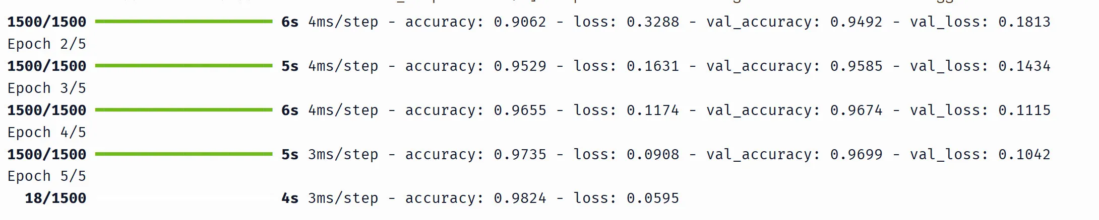
Here’s what each part means:

• 1500/1500 — 1,500 mini-batches completed out of 1,500 total (48,000 training images / 32 per batch). While training is in progress you’ll see this count up (e.g. 18/1500 means 18 batches done so far).
• 5s 4ms/step — the epoch took 5 seconds, ~4 milliseconds per batch
• accuracy: 0.9529 and loss: 0.1631 — training metrics, averaged over all batches in the epoch
• val_accuracy: 0.9585 and val_loss: 0.1434 — validation metrics, computed once at the end of the epoch on the held-out 12,000 images

The numbers from Keras and NumPy won’t be identical (different random weight initialization), but they should be close — both around ~97% validation accuracy after 5 epochs. This confirms that our from-scratch NumPy code implements the same algorithm as Keras.

What we’ve covered

We’ve taken every concept from the previous article and applied it to a real problem — classifying handwritten digits with 100,000+ parameters instead of fitting a line with 2:

1. Classification vs regression: softmax converts raw logits into probabilities, cross-entropy measures how wrong those probabilities are
2. Forward pass: input flows through layers, each computing $f(W\mathbf{x} + \mathbf{b})$ — same formula, now in matrix form
3. Backpropagation: the gradient of softmax + cross-entropy simplifies to $\mathbf{p} - \mathbf{y}$, and the chain rule flows backward through layers exactly as we derived by hand
4. Training loop: shuffle, split into mini-batches, forward pass → loss → backprop → update — repeated for every batch in every epoch

The algorithm is identical to what we built in the previous article. Keras automates it, but under the hood it’s the same computation our NumPy code performs step by step.

But we used the default settings throughout — one hidden layer of 128 neurons, learning rate 0.1, batch size 32. What happens if we change them? In the next article, we’ll systematically vary each piece — learning rate, batch size, network depth, activation functions — and explore overfitting, early stopping, and how to diagnose when training goes wrong.