What a trained MNIST classifier reads: row space and null space
A trained MNIST classifier represents each image with 128 hidden activations, but its final linear layer reads only ten independent directions. We can remove the other 118 directions without changing any digit score beyond floating-point roundoff. This experiment constructs that intervention and checks it on all 10,000 test images.
This article builds on Vector decomposition and subspaces: what a matrix reads and erases. That explainer develops vector decomposition and the four fundamental subspaces with small matrices and interactive diagrams. Here we’ll turn that geometry into an intervention: first construct a projection by hand, then build one from the learned weights.
In this article, we’ll focus on the null space: the directions in a learned representation that the output layer cannot detect. We’ll identify those directions in a trained MNIST classifier and construct a projection that removes their contribution, showing how we can reduce the representation’s independent directions without changing any output score or prediction.
We’ll use tools from linear algebra: singular value decomposition (SVD) to identify directions and how a matrix scales them, and projection to keep or remove selected components of a representation.
We’ll build on the dense network from training a real network on MNIST, which turns 784 pixel values into 128 hidden activations, then ten digit scores.
The part we’ll inspect is the output layer’s learned weight matrix, , which transforms the vector of 128 activation values produced by the hidden layer for one image () into digit scores. The weights are stored parameters shared across inputs; the activations in are values computed anew for each image. Applying SVD to tells us which directions in the hidden representation can affect the scores and which the output layer ignores.
The question guiding the experiment is: which changes to a learned representation are invisible to the classifier, and how can we remove those components without changing its predictions?
After training the network and freezing its learned weights, we’ll follow four steps:
- Discover what the output layer cannot detect: identify its null space from the trained weight matrix.
- Separate each representation into two components: a row-space component that determines the scores and a null-space component that contributes zero.
- Remove the undetectable component: construct a projection that keeps only the row-space component.
- Verify that predictions stay unchanged: pass the modified vector through the original output layer and compare its scores and predictions with the baseline.
Start with the trained MNIST network
We build the same architecture as the original article using PyTorch: one hidden layer turns 784 pixel values into 128 activations, and the output layer uses them to predict the digit. PyTorch supplies the layers, automatic differentiation, and optimizer; our intervention changes the activations between its two linear layers.
A vector is described by a list of numbers called its coordinates. In an image vector, each number is a pixel’s intensity. In our hidden representation, each coordinate is the numerical output of one neuron. It tells us how much of that coordinate direction contributes to the representation vector. Together, these values determine the vector’s direction and magnitude. The full MNIST network has 128 activations describing one vector in its 128-dimensional hidden representation space.
Here is the network used by the downloadable experiment:
import numpy as np
import torch
from torch import nn
from pathlib import Path
from classifier_subspaces import load_mnist

torch.set_num_threads(2)
torch.use_deterministic_algorithms(True)
torch.manual_seed(42)
model = nn.Sequential(
    nn.Linear(784, 128),
    nn.ReLU(),
    nn.Linear(128, 10),
)
Train once, then freeze the network
The loader comes from the downloadable classifier_subspaces.py in the reproduction section. It downloads the original MNIST arrays and caches them locally. We flatten each image, scale its pixels to , and keep integer digit labels:
(train_images, train_labels, test_images, test_labels), _ = load_mnist(
    Path.home() / ".cache/mirror-span"
)
train_x = torch.from_numpy(train_images.reshape(-1, 784).astype(np.float32) / 255)
train_y = torch.from_numpy(train_labels.astype(np.int64))
test_x = torch.from_numpy(test_images.reshape(-1, 784).astype(np.float32) / 255)
test_y = torch.from_numpy(test_labels.astype(np.int64))

optimizer = torch.optim.Adam(model.parameters(), lr=0.002)
generator = torch.Generator().manual_seed(43)
model.train()
for epoch in range(8):
    for indices in torch.randperm(len(train_x), generator=generator).split(512):
        optimizer.zero_grad(set_to_none=True)
        logits = model(train_x[indices])
        loss = nn.functional.cross_entropy(logits, train_y[indices])
        loss.backward()
        optimizer.step()

model.eval().requires_grad_(False)
model.double()
test_x = test_x.double()
feature_extractor = model[:2]  # Linear followed by ReLU
head = model[2]               # Linear: 128 activations -> 10 logits
The final layer returns raw scores. PyTorch’s cross-entropy loss expects these logits, so we do not put a softmax inside the network. loss.backward() computes gradients for both linear layers; optimizer.step() updates their weights and biases. After eight epochs, requires_grad_(False) freezes those parameters. eval() sets evaluation mode; it does not itself freeze weights. We cast the trained model and test inputs to float64 to measure the projection identities with less rounding error.
For one test image, the frozen network’s prediction follows two steps:
image = test_x[0]
with torch.inference_mode():
    h = feature_extractor(image)
    logits = head(h)
    probs = logits.softmax(dim=-1)
print(h.shape)      # torch.Size([128])
print(probs.shape)  # torch.Size([10])
The 128 values in are the hidden layer’s output and the output layer’s input. The output layer transforms these values into ten scores, or logits, using a trained weight matrix and a bias vector :
Softmax converts the ten scores into probabilities, and the largest probability determines the prediction. If we preserve all ten scores, we preserve the probabilities and prediction too.
We can see here that the output layer’s transformation matrix reduces the dimensionality from the 128-dimensional hidden space, , to the ten-dimensional output space, . It cannot preserve every independent direction in the hidden space, so different hidden vectors can produce exactly the same scores. The interesting question then is: which directions in the 128-dimensional hidden space carry information that the output layer uses to calculate its ten scores, and which does it ignore?
To find that out, we’ll freeze the trained network and insert a transformation between the hidden and output layers, changing only the vector passed to the output layer. This transformation will still return 128 numbers, but restrict them to ten independent directions—effectively removing the contribution of the other 118 directions—while preserving every output score. In our trained model, those 118 independent directions span the output matrix’s null space. We’ll manually construct the new transformation to remove the entire component in that subspace, which the output layer already maps to zero.
We will use the row-space and null-space decomposition from the companion explainer to construct that transformation from the learned weights.
From the subspace diagram to hidden activations
In the companion explainer, we drew the decomposition in three dimensions. Its blue vector now becomes the 128-number hidden representation computed for an image. The trained output matrix maps that representation to ten digit scores. Our measured matrix has rank 10, so the colors map to these spaces:
| Vector | Original matrix in the explainer | Trained MNIST output matrix |
|---|---|---|
| Blue | Full 3D input space | Full 128D hidden space |
| Green | 2D row-space plane | 10D row subspace |
| Pink (red) | 1D null-space line | 118D null subspace |
All three MNIST vectors still have 128 coordinates. The subspace dimensions count the independent directions available to each component, just as green in the explainer’s widget has three coordinates but is restricted to a 2D plane. The ten retained directions can combine many hidden activations; they do not have to coincide with ten individual neurons.
Our experiment performs the equivalent of clicking Remove null component: after training, we insert a projection before the output layer that keeps green and removes red. The ten digit scores stay the same because:
Here is the output layer’s fixed bias vector. We’ll also test the opposite intervention: keep only the null-space component and measure what happens to the predictions. Keeping only red gives , so the scores lose their dependence on the image.
We analyze the weights but intervene on the activations: each comparison uses the same input images and learned weights, so any change in prediction comes from the representation we pass to the output layer. The experiment checks both predictions numerically using learned weights and real MNIST images; score equality holds up to floating-point roundoff.
Build a projection that preserves the next matrix’s output
Before constructing the intervention for 128 hidden activations, let’s work through a three-coordinate example. The subspaces explainer showed how to split an input into the components a matrix reads and ignores. We’ll now turn that decomposition into a projection inserted before an unchanged output layer.
We’ll test both interventions on the small example: keep the row-space component and preserve the output, or keep only the null-space component and obtain zero. Then we’ll use SVD to construct the same interventions for the trained MNIST weights.
Use a matrix that reads the sum of the first two input coordinates and the third coordinate separately:
This matrix has row-space plane and null-space line , the same input subspaces as the explainer’s three-output example. Its outputs fill , so its left null space contains only zero. In the widget below, select an input basis vector to see its destination as a column of . Selecting and shows two different inputs reaching the same output.
Construct the projection from the component formula
The row-space component must have equal first and second coordinates while preserving their sum. Averaging those coordinates and keeping the third gives . The matrix that performs this operation is:
The projection returns three coordinates but restricts them to a two-dimensional plane. It removes an independent direction without deleting a coordinate. The two routes are:
This works for every input, not just our example. Multiplying the matrices gives:
Therefore . Adding the same output bias to both routes preserves the equality: .
Keep the erased component instead
Subtracting the projection from the identity extracts the other part:
For our input, . This matrix has rank 1: all its outputs lie on the null-space line. Passing them through gives zero because . With an output bias, only the bias vector remains.
In the widget, edit the input and choose what reaches the same output layer. Keeping the row-space component moves the input onto the green plane without changing its output. Keeping only the null-space component moves it onto the pink line and makes both outputs zero.
See the projection in two dimensions
The following animation makes the perpendicular motion easier to inspect. It uses a different projection, onto the orange line in direction :
Choose an example and press Animate projection, or drag the input:
- A vector perpendicular to the orange line, such as , maps entirely to zero.
- A vector on the orange line, such as , stays unchanged.
- Any other vector loses its perpendicular component and keeps its component along the orange line. For example,
Both components are two-coordinate vectors. The blue line is already the null space; vectors on it move to the origin, not into the null space. For this orthogonal projection, the orange line is both the row space and the column space. It preserves the difference between coordinates, whereas our three-dimensional projection preserves the sum of the first two.
Construct the projection for the trained 128-to-10 layer
Now apply the same process to the trained network: identify its output matrix’s null space, remove that component from each hidden representation, and verify that the scores stay unchanged. Freeze every learned weight and bias, and insert the projection after the hidden ReLU, before the existing output layer:
is the existing trained output matrix; is the extra matrix we construct. Keeping the row-space component means replacing with . The original output layer still receives 128 values, but those values are restricted to its ten-dimensional row space. These directions can involve all 128 coordinates; we are not selecting ten particular neurons.
The toy matrix above made the construction easy to see: one row reads the sum of two coordinates, and the other reads the third coordinate. The trained MNIST weights can mix all 128 coordinates with different positive and negative weights. We need a general way to identify the directions and build the projection. That is where SVD comes in.
| Toy experiment | Trained MNIST experiment | |
|---|---|---|
| Output matrix | ||
| Rank of | 2 | 10, measured after training |
| Inserted projection | ||
| Coordinates returned by | 3 | 128 |
| Independent directions retained by | 2 | 10 |
| Null-space directions removed by | 1 | 118 |
| Effect on output scores | Unchanged | Unchanged |
In general, rank plus nullity equals the input dimension:
Ten rows give a rank of at most ten; dependent rows could make it smaller. We measure rank 10 in our trained matrix, so the nullity is 118. The inserted row-space projection has the same rank and null space as .
Keep the spaces distinct: the row space and null space of live inside , where its input vectors live. Its column space lives in the ten-dimensional score space. Row and column spaces have the same dimension, but contain different kinds of vectors. The weight-matrix article develops these two views of multiplication.
Step 1: obtain the retained directions with SVD
For an introduction to SVD, see Singular Value Decomposition (SVD): Mathematical Overview. We apply it to the trained output-weight matrix:
The right singular vectors are columns of . Each has 128 coordinates and describes a direction in the hidden space. Its corresponding singular value tells us how strongly scales that direction into an output direction specified by . Those associated with nonzero singular values form an orthonormal basis for the row space: perpendicular unit vectors spanning all the hidden-space directions that can affect the scores.
We keep every nonzero direction, rather than selecting only a few large singular values. We do not need to collect activations to discover this subspace: it follows from the weights themselves.
In our trained network, SVD identifies ten retained directions spanning the row space. The perpendicular part of the 128-dimensional hidden space has 118 independent directions, which span the output matrix’s null space. Every vector in that null space satisfies , so its contribution to all ten scores is zero. These directions can involve combinations of many activations; they are not necessarily 118 individual neurons or coordinates.
Our inserted projection keeps the row-space component and removes the entire null-space component. The scores stay unchanged because the trained output layer already maps that removed component to zero. We do not need to calculate the 118 null-space basis vectors individually: constructing a projection onto the ten retained directions removes everything perpendicular to them. Its output still contains 128 coordinate values.
Step 2: turn those directions into a projection matrix
Put the ten retained directions into the columns of a matrix . To project a hidden vector, first measure its component along each direction, then rebuild it using only those components:
Equivalently,
The scalar measures how much of lies along direction . Multiplying by builds that component, and adding all ten components gives the projection. Those ten intermediate values are coordinates in the row-space basis, not the ten digit scores; the unchanged output layer still computes the scores afterward.
For comparison, our toy output matrix used rows and . Normalizing them gives
These are perpendicular unit vectors in the row-space plane. Putting them into the columns of a matrix and building produces the averaging projection we constructed above: . SVD supplies an orthonormal basis when the rows are not so convenient.
Here is the same construction for the learned weights:
# head.weight has shape (10, 128).
W = head.weight.detach().double()
_, singular_values, Vh = torch.linalg.svd(W, full_matrices=False)

# A numerical threshold determines which singular values count as nonzero.
tolerance = max(W.shape) * torch.finfo(W.dtype).eps * singular_values.max()
rank = int((singular_values > tolerance).sum())
Q = Vh[:rank].T                       # (128, 10) in our trained model
P_row = Q @ Q.T                      # (128, 128), rank 10
P_null = torch.eye(128, dtype=W.dtype) - P_row  # rank 118
Steps 3 and 4: intervene on the activations and check the scores
Apply the projection between the same feature extractor and output head. For a batch, PyTorch stores the hidden vectors as rows, so the column-vector formula becomes h @ P.T:
with torch.inference_mode():
    h = feature_extractor(test_x)     # (10000, 128)
    original_logits = head(h)
    row_logits = head(h @ P_row.T)
    null_logits = head(h @ P_null.T)

torch.testing.assert_close(row_logits, original_logits, atol=1e-10, rtol=0)
torch.testing.assert_close(
    null_logits, head.bias.expand_as(null_logits), atol=1e-10, rtol=0
)
assert torch.equal(row_logits.argmax(1), original_logits.argmax(1))
print((row_logits.argmax(1) == test_y).double().mean().item())
For the same image, the hidden layer still produces the same . There is no backward pass or weight update; only the vector passed to the output layer changes.
Every hidden vector splits uniquely into two perpendicular components:
Passing each component through the same output layer gives the two guarantees we will test:
The row-space projection preserves every score, hence every probability and prediction. The null-space projection leaves only the biases, giving the same probability distribution for every image. We retain 118 independent directions in that second condition, but none that this head can read.
The geometry is specific to this output layer. A direction it ignores might contain information another classifier could use. Likewise, the complete network is nonlinear: its original hidden activations need not form a subspace. The projection restricts them to one.
A projected hidden vector can contain negative values even though the original ReLU outputs are nonnegative. The inserted layer is linear; adding another ReLU before the final weighted sum would break the guarantee. The experiment uses float64 for projection and evaluation so roundoff is small. It casts the trained parameters once and uses the same values in every condition; it does not retrain them.
Why changing the representation need not change the prediction
The projection changes distances as well as coordinates. For two hidden vectors,
For a concrete three-coordinate example, take and . Their difference is , with length . It lies in the null space. Both project to , so their distance becomes zero, while both sets of scores remain .
More generally, the projection removes null-space differences and preserves row-space differences. Hidden-space distances can shrink while score differences stay exactly the same:
A large activation or distance therefore does not automatically mean importance to this prediction: the output layer may ignore that direction. Here we actively change vectors. Merely expressing the same vectors in a different basis would preserve both the vectors and their distances.
Methodology: identify, isolate, and intervene
In larger trained networks, knowing how to calculate every output does not automatically reveal what the internal representations encode or how the network uses them. Vectors provide a general way to encode objects, their properties, and relationships between them. The same mathematical tools can represent apple measurements for ripeness classification, image pixels for object recognition, or concepts and relationships for language understanding and generation.
Representational analysis studies what information internal vectors encode and how it is organized. Mechanistic interpretability investigates how a network’s components use that information to produce its behavior. The approaches overlap, but finding information in a representation does not by itself show that the network uses it.
A manageable approach to studying learned representations is to identify a candidate property, isolate its effects as carefully as possible, then test what changing its representation actually does. This experiment starts with a property we can define exactly: whether a hidden-space direction can affect the final layer’s scores. We are not yet trying to identify a semantic property such as color or stroke shape.
In mechanistic-interpretability terms, we combine weight analysis with a controlled intervention on activations. The tools serve distinct steps:
| Methodology step | Tool and its purpose |
|---|---|
| Identify the property of interest | Weight analysis: ask which hidden directions can change the scores, using the trained output matrix. |
| Isolate the relevant components | SVD and orthogonal decomposition: construct a row-space basis and split each hidden vector into components the layer can and cannot read. |
| Change only those components | Projection and activation intervention: keep the row-space or null-space component after the hidden ReLU. Keep the image and all learned weights and biases fixed. |
| Test the consequences | Paired evaluation: compare logits, probabilities, predictions, and accuracy on the same test images; check the algebraic identities and unchanged parameters. |
The implementation uses PyTorch to train and freeze the network, torch.linalg.svd to obtain the basis, and matrix multiplication to apply the projectors. Float64 evaluation and numerical assertions check score preservation and bias-only output. The interactive examples display recorded predictions from these evaluations.
We use PyTorch’s reduced SVD, with full_matrices=False, on the CPU. It computes all ten singular values of the weight matrix and their associated directions, while omitting extra basis vectors. This is a standard numerical decomposition, not an approximate algorithm that computes only a few leading directions.
The conclusion has an exact algebraic guarantee: we can prove score preservation or bias-only output before evaluating a single image. The experiment checks that our implementation obeys those identities. It identifies what this final linear layer reads, without assigning meanings such as “loop” or “stroke” to the directions or explaining how earlier layers learned them.
Four questions to carry into the next experiment
ValueShift Research’s How to Open Them Up – Part I separates four jobs when studying representations: finding them, establishing their causal role, testing their necessity, and steering behavior through them. Our linear-layer experiment is a useful starting point, with a narrower scope:
| Job | What this experiment establishes |
|---|---|
| Find a representation | SVD identifies the subspace the output layer reads. It does not identify a semantic concept such as a loop or a stroke. |
| Establish its causal role | Changing a null-space component cannot affect the scores; removing the entire row-space component leaves only the biases. |
| Test its necessity | Null-space components are unnecessary for this head’s output. Removing the whole row-space component eliminates image-dependent scores, but does not show that every retained direction is individually necessary for a correct prediction. |
| Steer behavior | Row-space projection preserves behavior; null-space projection makes it constant. Neither demonstrates a useful targeted correction. |
The colored-MNIST follow-up applies all four questions to a candidate property: color. It finds directions from controlled recolorings and tests whether suppressing or replacing their components changes the frozen classifier’s decisions.
What the experiment measures
We train the same dense architecture on MNIST’s original 60,000 grayscale training images and evaluate on the original 10,000 test images. We use seed 42, eight epochs of Adam, learning rate 0.002, batches of 512, and two CPU threads. This is a fresh reproducible training run with the earlier article’s architecture, not a claim to reuse its original saved weights or optimizer settings.
The full experiment was rerun on October 8, 2026, using Python 3.12.13, PyTorch 2.7.1+cpu, and NumPy 2.2.6 on Linux. The three-way comparison checks accuracy, all ten logits, probabilities, and per-image predictions. It also checks that the learned tensors stay unchanged, that both projectors are idempotent, and that the null-space output agrees with the bias vector.
| Representation | Independent retained directions | Test accuracy |
|---|---|---|
| Original hidden vector | 128 | 97.27% |
| Keep the output layer’s row space | 10 | 97.27% |
| Keep the output layer’s null space | 118 | 8.92% |
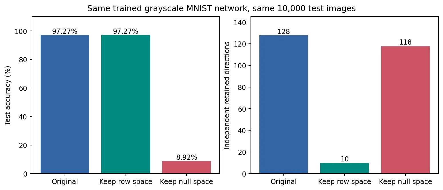
The learned output matrix has rank 10. Row-space projection changes zero predictions across all 10,000 test images. Its largest logit difference from the original evaluation is about , and its largest probability difference is about , consistent with floating-point roundoff.
Null-space projection makes the model predict 5 for every image: that class has the largest learned bias. Its 8.92% accuracy is the proportion of 5s in this test set, not random guessing. The largest difference between its logits and the bias vector is about .
All learned tensors remain bit-identical across the three conditions. Casting the trained model to float64 for evaluation changed none of its original predictions. This is one fixed training seed, but the algebraic guarantees do not depend on obtaining a particular baseline accuracy.
These checks separate the algebraic claim from any particular accuracy score. Row-space projection preserves the classifier’s existing mistakes too; it is not an accuracy-improvement technique. Null-space projection removes every image-dependent contribution this head can read, although the retained representation can still contain information for a different head.
This is why simply counting dimensions is insufficient. A small retained subspace can preserve every prediction, while a much larger one can make this classifier ignore its input entirely.
A separate question: can removing directions help?
The exact projection above preserves or destroys what the output layer reads. A different question is whether we can improve its decisions by suppressing directions it uses in a misleading way.
The independent experiment in when removing features improves a frozen classifier explores that question with colored digits. It estimates color-associated hidden directions and measures both the benefit under misleading colors and the cost under familiar colors. That result is empirical; the row-space and null-space identities here follow directly from the learned matrix.
Reproduce the experiment
Download the self-contained experiment script, offline tests, pinned requirements, and recorded results. Place the script, tests, and requirements in one directory:
python3 -m venv .venv
source .venv/bin/activate
python -m pip install -r requirements.txt
python -m unittest discover -s . -p 'test_classifier_subspaces.py' -v
python classifier_subspaces.py --quick
python classifier_subspaces.py
The requirements target CPU PyTorch on Linux. The script downloads MNIST on its first run, trains the baseline, freezes it, and evaluates all three representations. Results, an accuracy/dimension figure, a checkpoint, and the recorded examples are written to out-classifier/. The full run took about six seconds on the test machine. Use --quick for a separate 2,000-training-image / 1,000-test-image smoke test with two epochs and output in out-classifier-quick/.
The four offline tests passed: they check training updates, an inserted layer with frozen parameters, a rank-deficient output matrix, and a zero output matrix. The smoke test and full experiment also passed all numerical assertions. Those assertions compare scores and predictions, verify the projection identities, and confirm that the learned tensors remain unchanged. The Python snippets above were executed in order against the full dataset.
The JSON records the run timestamp, Python and library versions, dataset hash, seed, training settings, singular values, rank tolerance, accuracy, prediction changes, logit/probability errors, and geometry checks. The digit explorer uses recorded outputs for the first three test images of each digit. Its controls select those records; they do not run or retrain a network in the browser.