Removing and replacing features in a frozen classifier
In our first MNIST subspace experiment, we inspected the trained output matrix and removed the hidden representation’s component in its null space. The scores stayed identical because the output layer already mapped that component to zero. We could change the representation substantially without changing the classifier’s prediction.
Here we take the next step: what happens when we change components associated with a property the classifier may actually use? We’ll identify directions associated with color, then suppress their components or replace them with values from a differently colored version of the same digit. The predictions can now change; our question is whether those changes help or hurt.
A digit classifier can learn useful shape cues and a shortcut at the same time. If most training images of a particular digit share a color, color helps predict the label. When that association changes, the same learned shortcut can lead the network astray. This gives us a property to investigate and a concrete reason to intervene in its representation.
The part we’ll explore is the hidden layer’s output: the vector of 128 activations passed to the final classification layer. These activations are computed anew for each image; they are not weights. The learned weight matrices are stored parameters shared across inputs. We’ll collect hidden vectors for different recolorings of the same images and apply singular value decomposition (SVD) to their centered differences to identify color-associated directions. We then modify components of along those directions while keeping both layers’ learned weights fixed, and measure how the final scores and predictions change.
In this experiment, we train a small network on colored handwritten digits, freeze its learned weights, and insert a linear transformation just before its final classification layer. Removing two estimated color-associated directions improves accuracy on misleading colors from 85.91% to 90.59%, averaged over three training seeds. It also lowers accuracy on familiar colors from 98.09% to 97.16%. The intervention helps under one condition and costs accuracy under another.
We then keep the same selected directions and replace their components with values from recolored versions of the same images. This tests which changes in the digit probabilities can be produced by editing just those components, and how that compares with actually recoloring the input. Both experiments modify an already-learned representation; neither retrains the network.
From directions the classifier ignores to directions associated with color
Both articles use SVD to identify directions and insert a transformation between the hidden representation and the frozen output layer. The difference is which matrix we analyze and what its directions tell us:
| First experiment: the output layer’s null space | This experiment: color-associated directions | |
|---|---|---|
| Matrix we analyze | The trained output weights | Recorded activation differences caused by recoloring |
| Directions we identify | What the output layer reads and ignores | Where recoloring changes the hidden representation most |
| Intervention | Remove the component the classifier already ignores | Suppress or replace selected color-associated components |
| Consequence | Every score stays identical, guaranteed by | Scores and predictions may change; we measure whether that helps |
The color-associated directions are not assumed to lie in the output matrix’s null space. If they did, changing their components would leave every score unchanged. Only their components in the output matrix’s row space can affect its scores. Our intervention tests whether the directions we discover influence predictions and whether that influence is useful under different color conditions.
This is a new network trained on colored images, using the same kind of dense hidden layer and linear output layer. Within each experiment, we compare the same trained network before and after the intervention, with its learned weights fixed.
The task and the shortcut
Each input is a MNIST digit rendered in one of ten colors. Its label is still the digit, from 0 to 9. The network has a dense hidden layer with 128 ReLU activations and a final layer with ten digit scores. RGB gives it input values:
Colored image → 128 learned activations → ten digit scores → prediction
We assign one designated color to each digit. During training, we use that color with probability 0.9; otherwise we choose uniformly from all ten colors, including the designated one. The effective probability of the designated color is therefore 0.91.
We evaluate three conditions, using the same test digit shapes:
| Condition | Color rule |
|---|---|
| Familiar colors | The same association as training: each digit usually gets its designated color. |
| Independent colors | Color is sampled uniformly, independently of the digit label. |
| Misleading colors | Each digit usually gets the color designated for the next digit, wrapping 9 back to 0. |
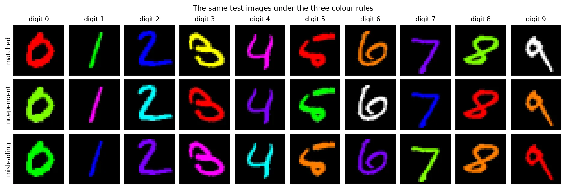
Each column shows the same source image under the three color rules. These are the first test images of each digit. Some colors can coincide because the rules include random sampling.
This is a ten-class Colored MNIST variant, inspired by the Invariant Risk Minimization experiments. We do not reproduce that paper’s binary task or its training method. Our question concerns an intervention in an already-trained network.
Change the learned representation, not the learned weights
For an image , the feature extractor produces a vector with 128 activations. The final layer computes
where contains ten digit scores. The largest score determines the prediction; softmax can convert the scores into probabilities.
After training, we freeze both parts. For suppression, we insert a matrix between them:
Same colored image → same feature extractor → inserted transformation → same classification layer
For a given evaluation condition, the image tensor and its original hidden activations are identical before and after insertion. Only the representation passed to the final layer changes. There is no further gradient update and no extra activation function after .
Compare recorded predictions before and after removing two color-associated directions.
Color: red
Test image #7
The projection changes hidden activations; it leaves this input image and every learned weight unchanged. Results are from seed 42, using a full rank-2 removal. Each digit is its first occurrence in the test set. Changing the color condition selects another recorded input, not a new training run.
The opening example in the explorer is a 9 that the frozen network predicts as 4 under misleading color. After projection, it predicts 9. Other examples remain correct, remain wrong, or become wrong. The full test set determines whether the intervention helps overall.
Find directions associated with color
We do not assume that a particular hidden neuron represents red, or that another represents digit shape. Instead, we measure what changes inside the network when the shape stays fixed and the color changes.
For an introduction to the decomposition we use, see Singular Value Decomposition (SVD): Mathematical Overview.
Here we discover candidate directions from the model’s responses to controlled input changes. The procedure is:
- Take 2,000 calibration images, separate from the training and test sets, and render each in all ten colors.
- Record the frozen network’s 128 hidden activations for each rendering.
- Subtract each source image’s average activation vector across its ten colors.
- Stack those differences into a matrix and apply singular value decomposition (SVD).
What does “record the activations” mean? The model stores its learned weights and biases, but computes a new representation for each input: . For one image, this is a vector of 128 numbers held in memory during the forward pass. Collecting these vectors as rows gives a representation matrix, with one row per input and one column per hidden activation. This matrix is computed data, not another set of learned weights attached to the layer, and it is not normally saved with the model. Here, we explicitly collect the representations for all 20,000 renderings, then subtract each source image’s mean representation across colors to build the matrix we analyze with SVD.
For image rendered in color , the centered activation is
Each difference describes a movement in hidden space associated with changing the color of the same digit. Stacking the 20,000 differences gives a matrix of shape . We decompose it as
Its leading right singular vectors, the columns of associated with the largest singular values, identify directions along which these differences vary most. Each vector has 128 coordinates because it lives in hidden-activation space. These are patterns across activations, rather than a list of individual neurons to switch off.
These selected directions span part of the row space of , the matrix of recorded activation differences. This is a different row space from that of the output weights : describes how representations vary under recoloring, while determines how representations affect scores.
This is also principal component analysis (PCA) of the centered activation differences. Within each image, the ten differences sum to zero, so the rows of have zero mean overall. The right singular vectors are therefore the principal-component directions; their squared singular values measure the variation captured along each direction. We center within each image so that the analysis follows changes associated with recoloring that image, rather than variation across unrelated digit images.
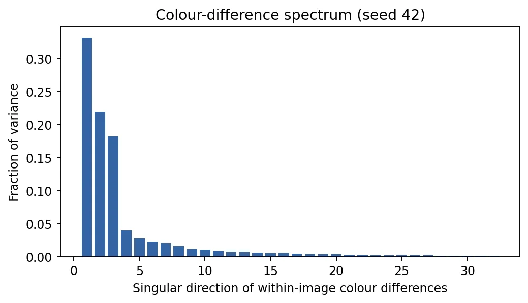
For seed 42, the first three directions account for about 73% of the squared variation in this calibration matrix. This does not mean they contain 73% of all color information, or that they are pure color features. The feature extractor is nonlinear: changes in color can affect responses to shape. We therefore call these estimated color-associated directions.
Insert a projection onto the remaining directions
Let the columns of be orthonormal directions chosen from that decomposition. The matrix projects a hidden vector onto their span. We insert
The parameter controls how strongly those components are suppressed:
- At , the layer is the identity.
- At , it halves the selected components. The transformation is still invertible and has rank 128: it changes their influence without erasing them.
- At , it projects them out completely. Its null space is the span of , and its output lies in the orthogonal complement. Its rank is .
At full strength, the null space of our inserted matrix is the selected color-associated subspace. Its row and column spaces are both the perpendicular complement: the directions we retain. In the first article, we constructed a projection whose null space matched what the trained output layer already ignored. Here, we construct a projection whose null space contains what we choose to suppress, then test the consequences for the unchanged output layer.
For the two-direction full projection, the layer still outputs 128 numbers, but those outputs have only 126 independent directions. The final classifier receives less information. At half strength, no direction is mapped to zero: the selected components shrink, but the transformation’s null space contains only the zero vector.
# U contains orthonormal hidden-space directions, shape (128, r).
A = torch.eye(128) - strength * (U @ U.T)

# For a batch, examples and hidden vectors are stored as rows.
with torch.inference_mode():
    h = feature_extractor(images)
    changed_h = h @ A.T
    logits = classification_layer(changed_h)
The runnable experiment also wraps this operation in an explicit fixed layer and checks that its logits agree with the direct calculation.
Scaling directions changes distances between examples
The transformation changes how far apart representations lie along selected directions. Write , where is the component in the selected color-associated span and is perpendicular to it. Then
For a small illustration, use two orthonormal axes: one selected color-associated direction and one perpendicular direction. These coordinates describe combinations of neurons, and the second axis is not assumed to represent pure shape. Consider two hypothetical representations:
| Intervention | First vector | Second vector | Distance between them |
|---|---|---|---|
| Identity | 2 | ||
| Half-strength suppression | 1 | ||
| Full removal | 0 |
The numbers illustrate the operation; they are not measured coordinates from our trained model. The perpendicular component stays fixed, while the selected difference shrinks and then disappears. Half strength preserves the possibility of recovering the original vectors by an inverse transformation; full removal merges them irreversibly.
For any pair of hidden representations, the same rule follows from linearity:
If , orthogonality gives the squared distance after the intervention:
Pairs that differ mainly along the selected directions move closer together. Pairs whose differences are perpendicular to those directions retain their distance. Removing two estimated directions does not guarantee that every recoloring of a digit becomes identical: color-associated differences can remain outside their span.
A general learned matrix can amplify, shrink, or redirect differences. Our inserted transformation specifically shrinks selected components while preserving perpendicular ones. This changes the balance of contributions reaching the frozen classifier. Whether it helps depends on what the classifier reads: its score difference for the pair becomes . Moving representations closer together is not, by itself, an improvement in classification. We measure predictions to find out whether the suppressed differences were helping or hurting under each color condition.
Methodology: identify, isolate, and intervene
Our experiment demonstrates a manageable piece of interpreting a network: identify a candidate property, isolate its effects as carefully as possible, then test what changing its representation actually does. Here the candidate property is color, which may supply a shortcut for digit recognition. We can change it while holding the source image’s shape and digit label fixed.
The first tool is a controlled input change: hold the digit shape fixed while changing its color, then inspect how the internal activations respond. SVD/PCA organizes those responses into candidate directions. At full strength, suppression is subspace ablation: remove the component of the activation vector in the selected span and observe how the frozen classifier behaves. At half strength, we attenuate that component instead. The replacement experiment adds activation patching: copy selected components from a donor forward pass into the source representation.
| Methodology step | Tool | What we do in this experiment |
|---|---|---|
| Identify the candidate property | A hypothesis about the training data | Test whether the learned association between color and digit contributes to errors when that association changes. |
| Isolate its activation effects | Controlled recoloring and within-image centering | Render each calibration image in ten colors, record its hidden activations, and subtract its mean across colors to form . |
| Estimate candidate directions | SVD/PCA of the activation differences | Find orthonormal directions capturing the largest recoloring-associated changes. Their meaning comes from the controlled experiment, not from SVD alone. |
| Choose what to change | Held-out validation | Select how many directions to suppress and by how much, without using the test labels. |
| Intervene in the representation | Orthogonal projection or partial suppression | Insert while keeping each evaluation image and all learned parameters fixed. |
| Replace rather than suppress | Activation patching within a subspace | Copy the selected coordinates from the same image in another color; preserve the source’s perpendicular component. |
| Test the consequences | Paired evaluation and random-subspace controls | Measure prediction changes and accuracy under familiar, independent, and misleading colors; compare selected suppression with random directions matched in rank and strength. |
The implementation uses PyTorch to record frozen hidden activations, torch.linalg.svd to decompose , and matrix multiplication for the inserted transformation. No separate concept classifier is needed to find the directions: the paired recolorings supply the comparison. Numerical checks verify the transformation and unchanged learned tensors; held-out accuracy measures whether it helps.
We use PyTorch’s reduced SVD, with full_matrices=False, on the CPU. It computes all 128 singular values of the activation-difference matrix and their associated directions; we select the leading directions afterward. This avoids constructing an unnecessary left-singular-vector matrix, but is not an approximate top-k SVD algorithm.
Large color-associated variation alone does not prove that a direction matters for predictions. SVD measures how much activations change; the final layer might largely ignore those changes. The intervention tests whether suppressing the selected directions changes decisions and accuracy. This makes the interpretation empirical, even though the projection itself has an exact mathematical definition.
Controlling the input property also does not guarantee a pure color representation. The network can respond to color differently for different shapes. Our claim is therefore limited to the estimated directions and their measured effects in this frozen model, rather than a complete account of its features or computation.
Choose the intervention without using test labels
MNIST’s original 60,000 training images are split into 50,000 for training, 5,000 for calibration, and 5,000 for validation. The original 10,000 test images remain held out. The color-direction estimate uses 2,000 images from the calibration split; it never uses the test images.
We evaluate candidate ranks and strengths 0.5 and 1. Selection maximizes mean accuracy across the three validation conditions. Rank 3 was added after inspecting the calibration spectrum; this exploratory change is recorded, and rank 3 was not selected in any run.
All three training seeds select two directions. Seeds 42 and 44 choose full projection; seed 43 chooses half-strength suppression. We report that selected intervention and the full projection at the same selected rank separately. The full projection is the condition that actually reduces the output span.
Inspect the validation behavior as more directions are removed
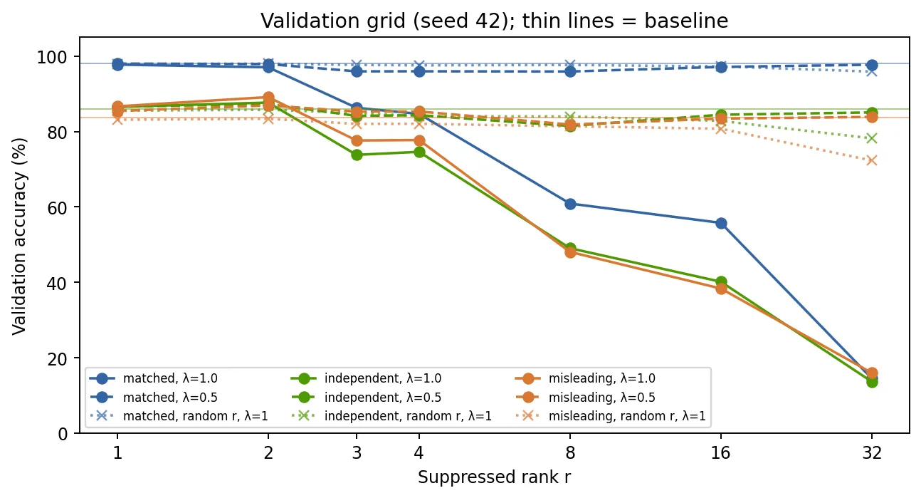
Removing more directions is not uniformly better. A decrease at rank 3 does not, by itself, identify the third direction as a specific shape feature.
What happened on the held-out images?
These are mean accuracies over training seeds 42, 43, and 44:
| Intervention | Familiar colors | Independent colors | Misleading colors |
|---|---|---|---|
| Original frozen network | 98.09% | 87.03% | 85.91% |
| Validation-selected suppression | 97.56% | 88.14% | 90.34% |
| Full projection of the same two directions | 97.16% | 87.58% | 90.59% |
| Random directions, matched to selected rank and strength | 98.06% | 86.92% | 85.88% |
The full projection improves misleading-color accuracy by 4.68 percentage points, at a cost of 0.93 points on familiar colors. Its misleading-color scores are 90.07%, 90.51%, and 91.20% across the three seeds, compared with baselines of 84.34%, 86.91%, and 86.49%.
The random control uses three random subspaces per seed, matching both rank and strength to that seed’s validation-selected intervention. It is the comparator for the selected-suppression row; because seed 43 selects half strength, it is not a uniform full-projection control. The random changes do not produce a comparable improvement.
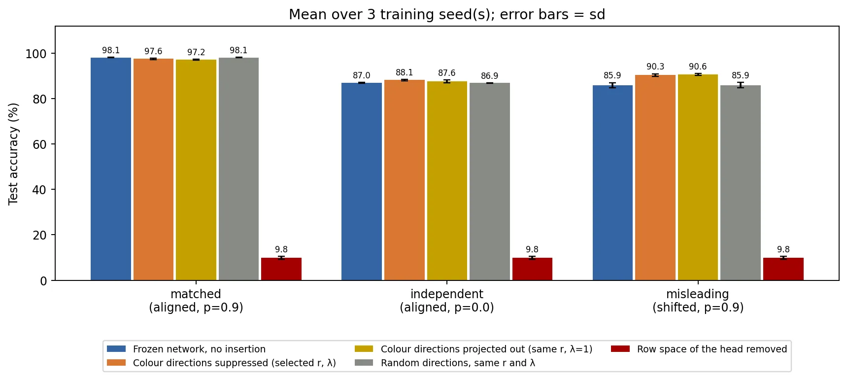
Error bars show standard deviation across the three training seeds. The JSON contains the per-seed results and full validation grid.
For seed 42, the selected intervention is a full projection. Under misleading colors it fixes 623 incorrect predictions and introduces 50 new errors. Under familiar colors it fixes 48 and introduces 120. These transitions make the tradeoff concrete: the transformation changes which mistakes the frozen classifier makes.
The independent-color score is not a measured “shape-only” score. Inputs are still colored, and the network can still respond to that color. It measures performance when color no longer predicts the digit label.
Replace components with values from another color
Suppression asks what happens when selected components shrink or disappear. Replacement asks what happens when we give them values from another forward pass. Take a source image, such as a red 9, and render that same handwriting in white. Run both images through the frozen feature extractor to obtain and . With , construct
We keep the source’s component perpendicular to the selected subspace and replace its two selected coordinates with the donor’s. The source image and learned weights stay unchanged. The donor has the same digit shape; we are not copying activations from a different handwritten digit. Its color can be one normally associated with another digit in training.
For a batch stored as rows, the operation is:
# Same frozen extractor, same shapes, different colors.
h = feature_extractor(source_images)
h_donor = feature_extractor(donor_images)

source_coordinates = h @ U
donor_coordinates = h_donor @ U
h_patch = h + (donor_coordinates - source_coordinates) @ U.T
logits = classification_layer(h_patch)
All three seeds use the two directions already selected by the suppression experiment. Replacement copies the donor coordinates completely; seed 43’s half-strength suppression setting does not apply. We do not choose a new rank or tune donor colors using test performance.
This intervention supplies information from another forward pass. For a fixed donor it is an affine transformation of the source vector: a projection plus an offset. Its outputs lie in a translated copy of the remaining 126-dimensional subspace, rather than necessarily a subspace through zero. It is not the same operation as removing information by projecting to zero.
Keep the source image fixed. Change only the hidden vector reaching the frozen output layer.
Stays fixed during the edit
Same shape, another forward pass
Copy only the donor’s two selected coordinates. Keep the source’s remaining 126 directions.
“Actual donor input” runs the recolored image through the whole network. It is a reference, not the result of the hidden edit.
Inspect the two selected coordinates
| Coord. | Source | Donor | Edited |
|---|---|---|---|
| c1 | -9.890 | -0.070 | -0.070 |
| c2 | 1.212 | 1.894 | 1.894 |
Coordinates in the selected SVD basis, not individual neuron values or RGB channels.
| Digit | Original | Hidden edit | Donor input |
|---|---|---|---|
| 0 | 0.01% | 0.01% | 0.00% |
| 1 | 3.93% | 2.15% | 0.00% |
| 2 | 0.07% | 0.08% | 0.00% |
| 3 | 1.82% | 0.62% | 0.00% |
| 4 | 51.27% | 24.74% | 0.00% |
| 5 | 1.95% | 6.84% | 0.00% |
| 6 | 0.07% | 0.04% | 0.00% |
| 7 | 0.59% | 0.15% | 0.00% |
| 8 | 3.18% | 2.37% | 0.00% |
| 9 (true) | 37.12% | 63.00% | 100.00% |
Recorded seed-42 outputs; first test image of each digit (this is #7). The basis and every learned weight stay fixed. Selecting the same source and donor color makes replacement a no-change check.
In the opening seed-42 example, the source red 9 is predicted as 4, with 37.12% probability assigned to 9. Copying the selected coordinates from its white rendering changes the prediction to 9, with 63.00% probability. Choosing magenta instead leaves the prediction at 4 and lowers the probability of 9 to 17.36%. The donor selector changes only which recorded coordinates we copy; the source image stays red.
Compare the patch with actual recoloring
The reference is the network’s output when it actually receives the donor image. We also test a complement patch: keep the source’s two selected coordinates and copy the donor’s component in the other 126 directions,
Together, these comparisons test whether the chosen subspace captures the prediction changes caused by recoloring. They do not assume that it contains all color information. The linear head makes the two patches’ logit changes add to the full recoloring change; probabilities and accuracy do not have that additive property.
For each of the 10,000 test images in each source color condition, we try all ten donor colors equally, including the original color. This gives 100,000 source/donor pairs per condition and seed, but still only 10,000 distinct source images. No digit label is used to choose the donors for these averages. Results below are mean accuracies across the same three training seeds:
| Intervention | Familiar source colors | Independent source colors | Misleading source colors |
|---|---|---|---|
| Original source | 98.09% | 87.03% | 85.91% |
| Remove the selected two directions | 97.16% | 87.58% | 90.59% |
| Replace the selected two directions | 95.75% | 85.01% | 88.34% |
| Replace the perpendicular 126 directions | 91.46% | 84.99% | 80.03% |
| Actually feed the donor image | 87.07% | 87.07% | 87.07% |
| Replace two random directions | 98.05% | 87.05% | 86.08% |
The actual-recoloring result is identical across columns because the donor images exhaust the same palette for the same shapes, regardless of source color. Random controls use three subspaces per seed, the same rank, complete coordinate replacement, and exactly the same donors. The removal row is repeated from the earlier experiment for comparison.
Replacement can help or hurt, and its behavior differs from both suppression and actual recoloring. Changes from patching the perpendicular component show that prediction-relevant color effects also exist outside the selected two directions. An accuracy difference alone does not quantify what fraction of color information lies in either part.
As a separate diagnostic using the known true labels, we can select the donor color associated with the true digit, or the color associated with the next digit. For misleading source images, replacing the selected components gives 92.96% accuracy with the true-digit donor color and 85.18% with the next-digit donor color. These are controlled comparisons, not methods for improving predictions on an unknown digit: choosing those donors requires its label. Both conditions were specified before measuring the replacement results.
Self-patching leaves logits unchanged. Numerical checks also confirm that the donor’s selected coordinates are copied, the source’s perpendicular component is preserved, and all learned tensors remain unchanged. Replacing the entire hidden vector reproduces the actual donor-image output; this is an implementation check, not an additional discovery.
What this establishes—and what remains uncertain
The learned tensors remain bit-identical throughout evaluation. The inserted layer is an actual hidden-space intervention, and its numerical checks agree with the intended matrix operations. As additional controls, keeping the final layer’s row space preserves its predictions, while keeping its null space makes the scores equal the biases, producing about 10% accuracy.
The measured suppression improvement shows that this trained classifier can make better decisions under misleading colors after selected directions are removed. It does not mean suppression creates information. It changes how the fixed classifier uses the information it already has. Replacement answers a different question: what happens when we supply selected components from a controlled donor? It requires that extra forward pass and need not reproduce the effects of changing the entire input.
Nor have we erased all color influence. Familiar-color accuracy remains substantially higher than independent-color accuracy after projection. The selected directions can mix responses to color and shape, and there is no guarantee that the same estimate, rank, or strength would work for another model. These results cover one architecture, one calibration size, and three training seeds.
The practical lesson is conditional: a direction that helps prediction under the training distribution can hurt when its association with the label changes. Suppressing it can improve a frozen model under the changed conditions, while making it worse under the original conditions.
Reproduce the experiment
Download the self-contained experiment script, pinned requirements, and recorded results. Put the script and requirements in the same directory:
python3 -m venv .venv
source .venv/bin/activate
python -m pip install -r requirements.txt
python colored_mnist_intervention.py
The requirements target CPU PyTorch on Linux. The first run downloads MNIST into ~/.cache/mirror-span/. The script trains with Adam at learning rate 0.002, batch size 512, for eight epochs per seed, with two CPU threads. The recorded full run, including replacement and its controls, took about 45 seconds. It writes results, four figures, seed-42 checkpoints, and example data to out-colored/. The JSON’s per-seed replacement entries contain all-palette and label-informed diagnostic results, random and complement controls, and numerical checks. Use --quick for a smoke test with separate output in out-colored-quick/.
The interactive examples use recorded seed-42 predictions for the first test occurrence of each digit. Selecting a digit, color condition, donor color, or intervention does not retrain or run a model in the browser. The pixel rendering and displayed predictions come from the same experiment export; replacement-samples.json also records the selected coordinates and all ten logits and probabilities for each comparison.