Anatomy of GPT-2: from text to token to output
A GPT model is two things at once that are hard to hold in your head together. From the outside it answers questions, writes code, and holds a conversation — it looks like it understands. From the inside it is a few hundred matrices and a loop that, given some text, produces one number per word in its vocabulary and picks one. The gap between those two descriptions is where most of the mystique lives, and it closes the moment you trace what actually happens to a prompt, step by step, all the way through.
This article traces one concrete model: GPT-2, the decoder-only counterpart to BERT. If BERT is the encoder branch of the architectural split — bidirectional, trained by filling in masked words — GPT-2 is the decoder branch: causal, trained to predict the next token and nothing else. We pick GPT-2 specifically because it is small enough to hold in one head (the original release ran from 124M to 1.5B parameters), fully public, and the model the best interactive visualizers actually animate. Wherever a stage has its own mechanics worth a chapter, we hand off to the deep dive rather than re-derive it here — most of all to the transformer-block teardown, which opens the one box this article is content to call “the blocks.”
The single most useful thing to fix before any of the parts make sense is what the machine is for.
The one job: predict the next token
Strip away the chat interface, the system prompt, the tool calls, and what remains is a function with one job: given a sequence of tokens, produce a probability distribution over which token comes next. That is the entire forward pass. “The cat sat on the” goes in; out comes a distribution that puts high probability on mat, lower on floor and rug, and almost none on purple. Sample one token from that distribution, append it, and run the function again. Generation is that loop — next-token prediction, over and over.
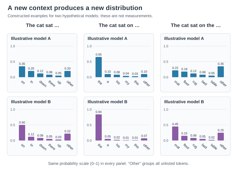
Each added token changes the context and triggers a new distribution. These constructed examples illustrate that change and possible differences between models; they are not GPT-2 or Mistral measurements. All panels use the same probability scale, and “other” includes every unlisted token.
This is the one place GPT and BERT genuinely diverge. BERT looks at a whole sentence at once and predicts masked words from both sides; GPT-2 reads strictly left to right and predicts the next word from everything before it. Same transformer block underneath — the difference is entirely in the attention mask and the training objective, which is exactly the bit the encoder/decoder article isolates.
Everything else is in service of making that one distribution good. Pretraining is the model learning to predict the next token over billions of tokens of text. The architecture — the part people mean when they say “transformer” — is just the specific shape of function that turned out to predict next tokens well at scale.
Framing it as a distribution is not a metaphor; it is literally what the model emits, and it is why the loss that trains it is cross-entropy / negative log-likelihood over a categorical distribution. The four building-block distributions that show up everywhere in deep learning — and why “predict a distribution, then minimize NLL” is the recipe behind classification, generation, and almost everything else — are the subject of a separate article; the categorical-over-vocabulary case is the one a GPT lives in.
Why GPT-2 mattered: scale is the multitask learner
BERT’s contribution was a new training objective. GPT-2’s contribution was the opposite claim — that you don’t need a new objective at all. Its paper title says it outright: Language Models are Unsupervised Multitask Learners. Take the single, boring objective above — predict the next token — and run it at enough scale on enough varied text, and the model starts doing tasks no one trained it to do. Prompt it with “translate to French: cat →” and it produces chat; prompt it with an article followed by “TL;DR:” and it summarizes. Nobody added a translation head or a summarization dataset. The tasks were latent in next-token prediction, because the training text already contained translations, summaries, and Q&A, and predicting those well requires doing the task.
That is the hinge the whole modern LLM era turns on. BERT said “train differently”; GPT-2 said “just make it bigger,” and the second idea is the one that scaled. Everything from here — the forward pass, training, inference — is in service of that one bet.
So the whole machine, top to bottom, is: turn text into a form the function can consume, run the function, read a distribution off the end, pick a token. Here is that pipeline end to end.
The forward pass, stage by stage
Six stages, one of which loops. The shapes matter as much as the names — most of the intuition for a GPT is “what shape is the data at each point, and what changed.” Click through the stages below; then we walk each one.
The prompt arrives as a Unicode string. The model never sees characters directly; the next stage turns them into integers.
A learned subword vocabulary splits the string into tokens and maps each to an integer id. Common words are one token; rare words split into pieces.
Deep dive: Tokenization: BPE, WordPiece, SentencePiece →Each token id indexes a row of a learned embedding table, turning 5 integers into 5 vectors of width d = 768. A learned positional embedding (one per slot) is added on top, so the vectors carry meaning and position — but no context yet.
Deep dive: Word embeddings & word2vec →The stack of N identical blocks (12 in GPT-2 small). Each block lets every token attend to itself and every EARLIER token (Q/K/V, multi-head, causal mask) and then transforms each position with a feed-forward network, wrapped in residuals + norm. Shape in = shape out; what changes is the content.
Deep dive: Inside a transformer block →The final vector of the last position is projected against the vocabulary to produce one raw score (a logit) for every possible next token. softmax turns these into a probability distribution.
Deep dive: The four distributions (softmax & NLL) →Pick one token from the distribution — greedily, or with temperature / top-k / nucleus sampling for variety. Append it to the input and run the whole pipeline again for the next token.
Sampling loops back to the start: the chosen token is appended and the full pass runs again, one token at a time. The KV cache is what stops this from re-reading the whole prompt on every step. Dimensions are illustrative (d = 768, N = 12, vocab = 50257 — GPT-2 small).
Tokenization: text → integers
The model cannot consume characters, and it does not consume whole words either. It consumes tokens — subword units from a fixed vocabulary learned once, before training, by an algorithm like BPE. GPT-2’s vocabulary is 50,257 entries of byte-level BPE. Frequent words (the, cat) are a single token; rarer words split into pieces (tokenization → token + ization); and because it works at the byte level, any string — emoji, code, garbage — always has a fallback. The output is a list of integer ids — [976, 9059, 7731, 402, 290] for our five-word prompt.
Why subwords and not words or characters is a real design decision with real consequences for vocabulary size, sequence length, and how the model handles typos and code. That trade-off, and the algorithms that dominate, are the tokenization deep dive. For the pipeline, the only thing to carry forward is: text in, a short list of integers out.
Embeddings: integers → vectors (plus position)
An integer id carries no meaning — 9059 is not “more cat” than 976. The embedding table fixes this. It is a learned lookup matrix of shape (vocab, d); each token id selects one row, a vector of width d (768 in GPT-2 small, up to 1600 in GPT-2 XL). Five token ids become a (5, 768) matrix.
These vectors are where “meaning becomes geometry” — tokens used in similar contexts end up with similar vectors, so direction and distance in this space encode relationships. That is the same idea word2vec made famous, and the word-embeddings article builds the intuition from scratch.
GPT-2 does one more thing here that matters: it adds a learned positional embedding. Attention, the next stage, has no inherent notion of order — without help, “dog bites man” and “man bites dog” would look identical. GPT-2 solves this the simplest way: a second learned table with one vector per position (slot 0, slot 1, …, up to its 1024-token context limit), added directly to the token embedding. So each input vector encodes what the token is and where it sits. (This is GPT-2’s actual scheme — learned absolute positions. Later models replaced it with rotary embeddings, RoPE, which is one of the things the block teardown and the modern-LLM follow-up cover.) One caveat the next stage resolves: the embedding is still context-free — at this point bank has the same vector in “river bank” and “bank account.” Making the vector depend on context is the transformer’s whole job.
Transformer blocks: vectors → richer vectors
This is the engine, and it is the one box this article deliberately does not open all the way — the “Inside a transformer block” article does exactly that, deriving each mechanism from the problem it solves. Here is the overview the rest of the pipeline needs.
A transformer block takes the (5, 768) matrix and returns a (5, 768) matrix — same shape, richer content. Each token’s vector comes out contextualized: bank now points in different directions depending on whether river or account sits nearby. A block does this with two sub-layers, each wrapped in a residual connection and a normalization:
- Masked self-attention is where positions talk to each other. Every token forms a query, a key, and a value (the Q/K/V projections); each token’s query is compared against the keys to decide how much to read from each, and the output is a weighted blend of values. Multi-head runs several of these in parallel (12 heads in GPT-2 small) so different heads can track different relationships. The decoder-defining detail is the causal mask: a token may attend to itself and every earlier token, but never a later one. This is what makes next-token prediction honest — the model can’t peek at the answer — and it is the single bit of architecture that separates GPT from BERT.
- The feed-forward network is where each position thinks for itself: a small two-layer MLP applied independently to every token vector, with no cross-position mixing. Most of the model’s parameters live here.
That block is then stacked N times — 12 in GPT-2 small, 48 in GPT-2 XL — each layer refining the representation a little more. Stacking identical blocks is the entire trick: depth is what turns “vectors that know their neighbors” into “vectors that have done something like reasoning.”
The reason attention is the expensive part, why it scales quadratically with sequence length, and why context windows top out where they do — all of that, plus the back-of-the-envelope math for parameter count (≈ 12·N·d²) and memory, is worked through in the block teardown and the inference-optimization article.
Logits and sampling: vectors → a token
After the last block, we have a contextualized vector for every position. For next-token prediction only the last position matters — its (768,) vector is the model’s summary of “everything so far, and what should follow.” That vector is projected against the vocabulary to produce one raw score — a logit — per vocabulary entry: a (50257,) vector of scores. GPT-2 does this with weight tying: the output projection reuses the input embedding table, transposed, instead of learning a separate matrix. The same (50257, 768) table that turns ids into vectors at the bottom turns vectors back into per-token scores at the top — fewer parameters, and a tidy symmetry. softmax turns those scores into the probability distribution we have been building toward.
Then sampling picks one token. The simplest choice is greedy — take the highest-probability token every time — but that produces flat, repetitive text. In practice you reshape the distribution first:
Logits are frozen; you are reshaping the distribution that the sampler draws from.Temperature < 1 sharpens it toward the top token (at the limit, greedy decoding);> 1 flattens it toward random. top-k keeps only the k highest tokens;top-p (nucleus) keeps the smallest set whose probability sums past p. Cut tokens (hatched) get zero mass and the rest renormalize. Values are illustrative.
Temperature divides the logits before the softmax: below 1 it sharpens toward the top token, above 1 it flattens toward uniform. Top-k keeps only the k most likely tokens; top-p (nucleus) keeps the smallest set of tokens whose probability mass clears a threshold. All three trade off coherence against diversity, and all three operate on the same frozen logits — they change which tokens the sampler is allowed to draw, not what the model believes. The chosen token is appended to the input, and the whole pass runs again for the next one.
That is the complete forward pass. Two questions remain: how the model’s weights came to produce good distributions (training), and how the generation loop is made cheap enough to serve (inference).
Counting the parameters
The block ledger counts about 12d² large-matrix parameters per conventional block. For GPT-2 small, d = 768 and 12 blocks give roughly 84.9 million. Token embeddings (50,257 × 768) add about 38.6 million, and learned positions (1,024 × 768) add about 0.79 million. With biases and normalization parameters the total is about 124 million. Weight tying means the vocabulary readout does not require another independent token-embedding-sized matrix.
The FFN accounts for two-thirds of the large-matrix weights inside each block, but embeddings remain a substantial part of this small model’s total. Attention’s mixing weights are computed activations and are not included in the parameter count.
How it learned: training
The forward pass above is fixed once the weights are set. Training is how the weights got there. For GPT-2 there is essentially one phase: pretraining. The model was shown a large web-text corpus (OpenAI’s WebText, ~40GB scraped from outbound Reddit links) and asked, at every position, to predict the next token; its prediction is compared to the actual next token with cross-entropy loss, and the error is pushed backward through every layer to nudge every weight. That backward pass is backpropagation — the chain rule applied mechanically through the whole computation graph — and the reason it works at all is that every operation in the network is differentiable, which is a deliberate constraint on what the architecture is allowed to contain. How the gradient actually flows through the stacked blocks (and why residual connections matter so much for keeping it alive at depth) is covered in how gradients flow.
Gradients tell you which direction to step each weight; the optimizer decides how far. Plain SGD, momentum, and Adam are different strategies for turning a noisy stream of gradients into stable steps, and the choice has a large effect on whether a model trains at all — the optimizers article walks through them.
The product of pretraining is a model with broad capability but no manners: GPT-2 is a next-token predictor, not an assistant. Prompt the raw model with a question and it will happily continue with three more questions, because that is what the text it saw tended to do. GPT-2 is exactly this raw base model — that is the whole point of it as a teaching example. The step that turns such a base model into something that answers rather than continues — post-training: supervised fine-tuning on instruction–response pairs, then preference tuning (RLHF and its descendants) — came after GPT-2, in the InstructGPT/ChatGPT line. Capability comes from pretraining; behavior is sculpted later. The frontier of that later phase, including on-policy distillation, is the subject of the on-policy distillation article.
How it runs: inference
A trained model is a pile of weights and the generation loop from the forward-pass section. Running that loop efficiently is its own engineering problem, and two ideas carry most of the weight even for a model as small as GPT-2.
The KV cache is the one that makes autoregressive generation tractable. Recall that generation appends one token and re-runs the pass. Naively, that means re-computing attention over the entire prompt at every single step — quadratic waste. But the keys and values for past tokens do not change when a new token is appended, so they are computed once and cached. Each new step computes Q/K/V for only the new token and attends against the stored cache. The cost is memory: the cache grows with context length. Why this is the inference bottleneck, and the schemes that shrink it (grouped-query attention and friends — modern additions GPT-2 itself predates), are the KV-caching and GQA deep dives.
Quantization attacks the weights’ memory footprint. Storing weights in INT8 or INT4 instead of FP16 roughly halves or quarters the memory and speeds up the memory-bound parts of inference, at a modest and often negligible accuracy cost. Why low precision works, what actually breaks when you push it too far, and how precision interacts with multi-GPU inference are covered in the precision and multi-GPU article. The full serving toolkit — continuous batching, paged attention, speculative decoding — is the inference-optimization article.
The shape worth remembering: weights scale with parameter count, the KV cache scales with context length, and compute scales with both — the same arithmetic the transformer-block article derives from the block dimensions.
The whole machine in one view
GPT-2 is not one inscrutable object. It is a chain of transformations, each of which does a small, nameable thing:
- Tokenization turns text into a short list of integers from a 50,257-entry byte-level BPE vocabulary.
- Embeddings turn each integer into a learned vector and add a learned positional vector for its slot.
- Transformer blocks — stacked N times — contextualize those vectors, every token attending to itself and every earlier token (the causal mask) and then being transformed position-wise. This is the engine; the block teardown opens it fully.
- Logits and softmax turn the last vector into a probability distribution over the whole vocabulary, reusing the embedding table (weight tying).
- Sampling picks one token, which is appended and fed back in — the generation loop.
- Training (pretraining for capability) is how the weights came to make that distribution good; inference machinery (KV cache, quantization, batching) is how the loop is made cheap to serve.
Nothing in that list is magic, and nothing in it is beyond following one step at a time. The best way to cement it is to watch the transformations move: Brendan Bycroft’s 3D LLM visualizer animates a real GPT (including GPT-2) forward pass layer by layer with every tensor shape laid out, and Roy van Rijn’s interactive “Anatomy of an LLM” lets you push the sliders on temperature and sampling and see the distribution respond.
GPT-2 is the original concrete decoder. Almost every model since is a variation on this exact pipeline with a handful of upgrades — RoPE instead of learned positions, RMSNorm, SwiGLU, grouped-query attention, mixture-of-experts — bolted onto the same text-in, distribution-out, token-appended story. What changed, why, and how much it actually matters is the subject of the follow-up on modern LLMs. From here you can either open the engine — the “Inside a transformer block” article derives attention, multi-head, the FFN, positional encodings, and residual + norm from scratch — or step back up to the encoder branch to see how the other half of the split spends the same machinery.