Understanding residual connections: identity and learned updates
The transformer architecture behind many of today’s LLMs brings together two closely connected parts: transformer blocks, which perform the computation, and the residual stream, which acts like a working memory for each token. The stream carries each token’s evolving representation from layer to layer. Inside each block, attention and feed-forward layers read this state, compute updates, and add them back, allowing later layers to build on earlier computation.
These updates are added through residual connections, which carry an existing representation forward and combine it with a learned update. Popularized by ResNet in 2015, residual connections became a standard component of deep neural networks. In transformers, they connect attention and feed-forward computations to the shared residual stream.
In this article, we’ll examine the problem that motivated ResNet, when an identity mapping preserves a working computation, and how a shortcut lets a branch learn an update. We’ll work through small vectors and matrices, then put the same mechanism inside a CNN. This will provide a foundation for future explorations of how different components use learned reading and writing directions within the shared residual stream.
How more layers made things worse
A plain network stacks layers in sequence, with each layer processing the previous layer’s output. Adding layers gives the network more steps to transform its input, yet the original ResNet paper showed a surprising result: a plain 56-layer network had higher training error than a plain 20-layer network on CIFAR-10. Even after training, the 56-layer network made more mistakes on the training data than the 20-layer network. This worsening of training performance with added depth was called the degradation problem.
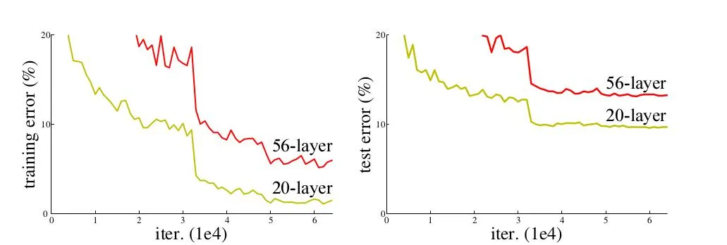
The left panel is the crucial evidence: the deeper network fits the training examples worse. The right panel shows that it also performs worse on unseen test examples, but the higher training error is what rules out overfitting alone as the explanation. Both networks here are plain networks, without residual shortcuts.
To see why this was surprising, imagine a network with one trained layer. Now add a second layer after it. We would expect the two-layer network to be capable of doing at least as well: if the new layer has nothing useful to contribute, it could simply pass its input through unchanged—a behavior called an identity mapping. With the first layer’s weights kept the same, the network would then produce exactly the same result as before.
Let’s demonstrate this idea using linear layers with no biases or activation functions. We start with one layer, which transforms the input into . Then we add a second layer, which receives and produces . If we want to preserve the original output, our new layer must pass through unchanged: .
Suppose the existing layer produces:
This means the added layer must learn the identity matrix, which leaves every input vector unchanged. It has ones on the diagonal and zeros everywhere else.
To demonstrate that the identity matrix leaves unchanged, we’ll compute the product using the row and column views introduced in Feature detectors: how neurons read and write. In the row view, we take the dot product of each matrix row with , selecting the corresponding input coordinate:
In the column view, we multiply each matrix column by the corresponding coordinate of and add the resulting vectors:
This works for every input vector, not just this example. With , the extra layer leaves the representation unchanged, so the rest of the network receives exactly what it would have received without that layer.
However, manually choosing weights that preserve the input is different from finding them through training. We chose ones on the diagonal and zeros everywhere else ourselves. A new layer’s weight matrix typically starts with random values, so it initially changes the representation. From that random starting point, preserving every input exactly would require training to reach the identity matrix we wrote down.
We could also initialize this plain linear layer directly with . It would then preserve the input from the start, and training could adjust the weights to make useful changes. If the desired transformation is close to identity, this can provide a starting point closer to the desired weights. Fewer required changes, however, do not automatically mean fewer gradient-descent steps.
With one added linear layer, preserving every input requires its weight matrix to be the identity matrix. With several added linear layers, their matrices must work together so that their combined transformation leaves the input unchanged. For example, if we add two layers after the original layer , their weight matrices must satisfy:
Setting each added matrix to is one solution; other combinations can also have an identity product. With the original network’s weights and operations unchanged, the added layers would then preserve its predictions.
Changing one layer’s weights changes what the following layers receive, so training must coordinate their effects. Adding more layers can make this optimization harder, even though we can manually choose weights that preserve the original result.
Why finding the weights can be difficult
In a real network, we want the added layers to improve the predictions. Preserving their input is a hypothetical fallback: if they contribute nothing useful, they could at least leave the existing result unchanged. The identity matrix shows that this fallback is possible. However, while preserving the input looks simple when we choose the weights ourselves, gradient descent can struggle to find a solution that performs even that well.
To understand what a residual shortcut changes during training, let’s first trace how gradients pass backward through our two-layer network. Each multiplication takes two inputs: a weight matrix and a vector. The first produces , the second produces , and a loss compares the output with a target . The solid arrows below show this forward computation. The dashed arrows trace gradients backward, with denoting the gradient of the loss with respect to .
To reach , the gradient is multiplied by ; to reach , it is then multiplied by . The superscript denotes the matrix transpose. These are gradients with respect to the representations. The gradients used to update the weights also use the inputs saved during the forward computation:
So even the update to depends on through . Adding more layers extends this chain of matrix multiplications. In nonlinear networks, activation derivatives enter the chain as well. Repeated multiplication can shrink gradients until earlier layers receive very small updates—vanishing gradients—or amplify them enough to make updates unstable—exploding gradients. Whether this happens depends on the weights, activations, and inputs; depth alone does not guarantee either outcome.
Yet, even when gradients are neither too small nor too large, training can still make slow progress because each layer’s effect depends on the others. The ResNet authors observed degradation even when gradients were not vanishing, so gradient magnitudes alone did not explain the difficulty.
Our example separates what the network can represent—expressivity—from what training can discover—optimization. The degradation problem exposed a difficulty with optimization: deeper networks could represent solutions as good as their shallower counterparts, yet training reached worse results. ResNet addressed this by adding shortcuts that carry representations forward while learned branches compute updates. Its experiments showed that this change helped training make effective use of additional depth.
Let the shortcut preserve the input
ResNet’s hypothesis was that learning an update to an existing representation could be easier than learning the complete transformation, especially when the desired result is close to the input. A shortcut carries the input forward, while the learned branch computes what to add. If nothing needs to change, the branch only needs to produce a zero update.
Let’s see how this idea applies to our example with one added layer, . Its input is , and we’ll call its output . The paper proposed adding a shortcut, also called a skip connection. In our example, it bypasses the added layer, carrying unchanged and adding it to :
In the illustration, layer 2 and the curved shortcut both receive the same input . Layer 2 computes the update , while the shortcut carries unchanged, bypassing the layer. Note that the identity shortcut is not a learned layer: it has no weight matrix to train. The two paths meet at the plus sign, where their outputs are added element by element, giving . For this addition, must have the same shape as .
Returning to our example, suppose we want the added layer to leave the original result unchanged. The shortcut already carries , so the layer only needs to produce a zero update:
For our vector, the computation becomes:
In the plain network, , so preserving every input requires . With a shortcut, , so preserving every input requires . The ones on the identity matrix’s diagonal are now supplied by the shortcut; the learned matrix only specifies what to add.
Without the shortcut, the added layer must learn to reproduce its input. With the shortcut, it only needs to produce a zero update to preserve it.
In PyTorch, the shortcut is simply the addition h + update. The linear layer stores in layer.weight; bias=False matches our example with no bias term:
import torch
from torch import nn

h = torch.tensor([2.0, 5.0, 3.0])
layer = nn.Linear(3, 3, bias=False)  # The added layer W₂

# Choose a zero update to demonstrate identity behavior.
nn.init.zeros_(layer.weight)

update = layer(h)  # F(h) = W₂h
y = h + update    # The skip connection

print(update.detach())  # tensor([0., 0., 0.])
print(y.detach())       # tensor([2., 5., 3.])
We explicitly set the weights to zero here; nn.Linear normally initializes them randomly. The shortcut itself needs no separate module or learned parameters—it is the original h in h + update. The layer’s weights remain trainable, so training can change the update when that improves the predictions.
Why learning an update can be easier
In the plain network, the added layer must produce the entire next representation. That includes both the values that should change and those that should stay the same. With the shortcut, the input already reaches the output through a fixed path. The learned layer only has to supply the difference between the input and the desired result.
The authors hypothesized that, when a useful transformation is close to identity, learning the required change would be easier than learning the complete transformation. Our matrix example illustrates this reformulation, but does not prove that gradient descent will converge faster. The evidence came from experiments with deep nonlinear networks, where residual connections improved training.
During training, we do not supply the branch with a correct update to copy. We train the whole network using its final task loss. Backpropagation adjusts the residual branch’s weights so that its updates help reduce that loss.
Next, we’ll examine another concrete change introduced by the shortcut: the additional path it provides for gradients. In our earlier plain computation graph, the gradient reaching had to pass through . The graph below separates the forward computation on the left from the backward gradients on the right. With the shortcut, the addition sends the output gradient along both paths, and their contributions add at .
Comparing the gradient reaching in the two arrangements:
The extra reaches directly through the shortcut, without being multiplied by . This provides a route for gradients even when the learned branch contributes very little. The same principle applies to nonlinear branches, although their derivatives determine the other contribution. The two contributions can still reinforce or cancel each other. The follow-up paper Identity Mappings in Deep Residual Networks analyzes these paths and tests their importance in deep networks.
This shows how the shortcut changes the gradient paths, but our single-layer example has a limit. Because , an ordinary linear layer can represent exactly the same computation. In particular, initializing the plain layer’s matrix to gives the same starting transformation as initializing the residual branch’s matrix to zero. With these equivalent starting transformations and the same learning rate under ordinary gradient descent without regularization, the two parameterizations train equivalently. The benefit demonstrated by ResNet concerns deep nonlinear networks, where the shortcut bypasses a sequence of learned operations.
Identity initialization chooses the starting weights. A residual shortcut provides a fixed identity path that remains available as the branch’s weights change. For a branch containing several layers and nonlinear operations, initializing each weight matrix to identity may not preserve the input through the whole branch. ResNet’s experiments demonstrated that its shortcut design could train deeper networks successfully. Updates need not always be small, but preserving a useful representation no longer requires the learned branch to reproduce it.
We can see that benefit in the paper’s ImageNet comparison. Here the researchers compared networks with 18 and 34 layers, both with and without residual shortcuts:
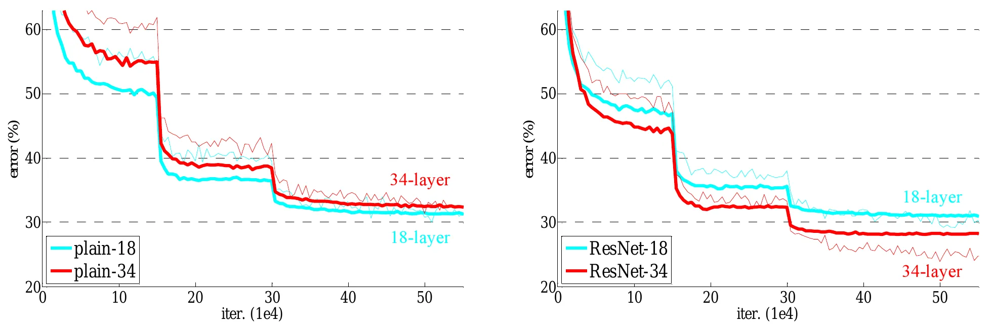
In the plain networks, adding depth made training performance worse. With residual shortcuts, the result reversed: the 34-layer network reached lower training error than the 18-layer network, and the improvement also appeared on the validation data. The residual networks in this comparison added no parameters to their plain counterparts. This is experimental evidence that the shortcut helped training make use of the extra depth.
When the added layer should change its input
So far, we’ve used the shortcut to preserve the input. Now let’s see what happens when the added layer needs to learn a useful change. Using the same input vector, we want to change the middle coordinate from to while preserving the other two. We’ll compare what the layer must produce with and without the shortcut.
Our input and desired output are:
First, let’s see how a plain layer can produce this change. Its matrix must produce the full output vector, preserving the first and third coordinates while changing the second. One matrix that does this is:
Multiplying this matrix by gives the plain layer’s output:
Now let’s produce the same output using a residual skip connection. The shortcut already carries the original input, so the layer only needs to supply the change: add to the second coordinate and leave the others untouched. Its output should therefore be . We can produce this update with the following matrix:
The layer computes the update, then the shortcut adds the original input:
Compute the update
Add the input
We can obtain the residual matrix by subtracting the identity matrix from the plain matrix. Matrix subtraction works element by element: we subtract corresponding entries of matrices with the same shape.
The diagonal ones disappear because the shortcut now supplies the unchanged input. The remaining matrix supplies the update. The plain layer and the complete residual block implement the same total transformation: the plain layer produces directly, while the residual branch produces and the shortcut supplies the rest.
This difference gives residual learning its name: the branch learns the change , while the shortcut supplies the input . In our example, the required change is . The residual is the change added to the existing representation.
We can illustrate the same idea with an image, where each coordinate represents a pixel’s brightness. Suppose is a blurry grayscale image and is the sharp version we want. The shortcut carries the blurry image, while the branch supplies the changes in brightness needed to sharpen it: .
Let’s inspect three pixels to see how adding the correction brightens one, darkens another, and leaves a third unchanged. Brightness ranges from 0 to 1.
| Pixel | Input | Correction | Result |
|---|---|---|---|
| Brighten an edge | 0.388 | +0.512 | 0.900 |
| Darken a window | 0.541 | -0.441 | 0.100 |
| Keep the background | 0.100 | 0.000 | 0.100 |
The correction increases brightness at some pixels and decreases it at others. Pixels that already match the target need no change. Adding positive values everywhere would simply brighten the image; restoring its boundaries requires signed updates.
This illustration calculates the desired correction directly from the input and target. A trained reconstruction model would instead predict it from the blurry input, using the sharp target only to compute the training loss. Inside a classifier or transformer, the values being updated are feature activations or token representations rather than visible pixels.
A shortcut can span more than one layer
Our single-layer example showed how the shortcut lets a layer produce an update. To see how this works in a ResNet, we need one extension: a single shortcut can bypass several learned layers together. We’ll show two here because the CNN block later in the article uses two convolutions to compute one update.
Keep as the input, but now let it pass through a linear layer, ReLU, and a second linear layer. Their combined output is :
Conceptually, we group the two layers and ReLU into one learned branch that computes a single update. Together with the shortcut, this forms a residual block. The diagram below shows the shortcut carrying around the entire branch:
The shortcut carries the input of the first layer directly to the addition after the second. There is no residual addition between the layers: the whole sequence computes one update, which is added to once.
Inside the branch, the layers can use a different number of coordinates. For example, could map our three input values to six, and could map those six values back to three. Their matrix shapes would be and , respectively. The intermediate representation can be wider; the final update must match so the two can be added.
ReLU acts between the matrices, replacing negative values with zero without changing the number of coordinates. This nonlinear step means the branch generally cannot be reduced to a single matrix multiplication.
Even with this extra computation, a zero update still preserves the input: . In our example without biases, setting the final matrix to zero is enough to make the whole branch output zero, while can still contain nonzero weights.
Later blocks read earlier updates
So far, we’ve followed the update produced by one residual block. When we stack blocks, each one receives the result of the previous block—including its update. This means an earlier block can change what a later block computes.
Let’s see this with our vector and two residual blocks, each with its own residual connection:
In the diagram below, the first block produces , which becomes the input to both paths in the second block:
Notice how the second branch reads the updated vector , not the original input . Both paths in the second block receive the result of the first block.
To keep the arithmetic simple, we’ll use linear branches. The first block adds the input’s first coordinate to its second; the second block subtracts its current second coordinate from its first. For an input , their branch updates are:
The first branch repeats our earlier example: it produces , which is added to to give . The second branch reads this updated vector and produces , subtracting the current middle coordinate from the first:
| Block | Vector it reads | Update it computes | Vector after addition |
|---|---|---|---|
| First | |||
| Second |
The interactive plot below shows both updates: the first moves our vector from to , and the second takes it to . The plot is a 2D projection of our three-dimensional vectors: the horizontal axis shows the first coordinate, and the vertical axis shows the second. The third coordinate stays at throughout, so this view shows every change made by the two updates.
As an experiment, turn off to force its update to zero. The second branch now receives and adds , giving . Removing the first update also changes the second update, so the new result is not simply the original final vector minus the first update.
If you tried disabling the first branch, you noticed that the second branch’s update changed too. This happens because the second branch reads , which includes the first update. Substituting into makes this dependency visible:
The first update appears both as something we add and as part of the input to the second branch. Changing it can therefore change both contributions to the final result.
With more residual blocks, we repeat the same process: each branch reads the current representation, computes an update, and adds it back. This sequence of updates can be described by a single formula. After residual blocks:
The standalone is our starting vector. The sum collects all the updates, but each update is computed from a different stage of the representation: reads , reads , and so on. The formula summarizes a sequence of dependent updates; it does not mean every branch operates on the original input. It assumes each block passes the result of directly to the next block. If it applies ReLU or normalization to that result first, we must include that extra operation in the formula.
In a transformer, this evolving representation is called the residual stream. Each residual block can use convolutions, attention, or an MLP to compute its update, provided that update has the same shape as the representation it is added to.
Put the shortcut inside a CNN
We can now apply the same idea to a CNN. Instead of a vector with three coordinates, we’ll use a stack of feature maps as the input . Suppose this stack contains 32 maps, each . Using the height × width × channels convention from our CNN article, this gives a tensor with shape 28×28×32 for one image.
First, consider a plain sequence of two convolution stages. The input passes through every operation, and the layers must produce the complete next representation. Both convolutions use 32 output channels, stride 1, and padding 1 to preserve its shape:
Now let’s add a residual connection around these two convolution stages, following the basic block design in ResNet18 and ResNet34. Its learned branch computes an update using two 3×3 convolutions, each followed by batch normalization, with a ReLU between the two convolution stages. The residual connection carries the same input around this branch and adds it to the update.
The diagram below follows Torchvision’s BasicBlock layout, using 32 output channels, stride 1, and padding 1 in both convolutions. These choices keep the update’s shape at 28×28×32, matching so the two can be added:
The residual connection bypasses the entire learned branch: both convolutions, both normalization operations, and the first ReLU. There is no ReLU immediately before the addition, so the branch can supply negative updates as well as positive ones. The final ReLU acts on the sum .
The block uses convolutions to compute an update of the same shape. The residual connection carries unchanged, and the addition combines each activation with its corresponding update. At row , column , and channel :
For example, an activation of plus an update of becomes . This happens across all 32 feature maps, leaving the tensor’s shape unchanged. The convolutions compute the changes; the residual addition applies them to the existing representation.
The final ReLU adds a qualification to our identity argument. This block computes:
If , the result is . That preserves a nonnegative input, as normally received from the preceding block’s final ReLU, but clips negative entries in an arbitrary signed input. Later work on identity mappings examined arrangements that leave the path after addition unchanged.
Our example keeps the input and update the same shape so they can be added directly. If a block changes the shape, the residual connection must also adapt the input—for example, using a learned projection. In that case, it no longer carries the input unchanged.
From residual connections to the residual stream
So far, we’ve viewed a residual connection as a path that carries the input around learned layers and adds it to their output. We can describe the same computation from another perspective—one that focuses on the evolving representation, rather than the individual skip connections. Each block reads the current state and contributes an update, which becomes part of the state passed to later blocks. This running state is what is called the residual stream.
The diagram below redraws two of our CNN blocks to emphasize this view. Follow the blue path downward: each local skip connection bypasses one convolutional branch, while the state continues through the whole sequence.
In the diagram, each skip connection is a local segment of the blue path: it carries the current state around one convolutional branch to the addition. Following the blue path through both blocks shows the residual-stream perspective—the representation evolves as successive blocks contribute updates.
The first addition combines with , then ReLU produces . The second branch reads this updated state and computes . In this ResNet layout, the evolving representation therefore reflects both the learned updates and the ReLU operations applied after each sum.
One evolving representation per token
Residual connections also appear in architectures beyond CNNs. One of the best-known examples is the transformer architecture, where the evolving representation is commonly called the residual stream. Let’s briefly see how the representation changes when we apply this pattern to a sequence of tokens.
In our CNN example, the representation contained a vector at each spatial position: 32 values, one from each feature map. In a transformer, it instead contains a vector for each token in the input sequence—the model’s context. During the forward pass, each transformer block reads from and writes to these representations in the residual stream. Attention reads information from the permitted token positions and writes an update to each token’s vector. The MLP then reads each updated vector and writes another update. The resulting representations pass to the next block.
The diagram below shows a pre-norm transformer block, where normalization sits inside the update branches. Read it from top to bottom. The blue path carries the sequence representation through both additions. Attention reads a normalized copy of ; the MLP reads a normalized copy of the updated state . Each branch returns one update vector per token.
The diagram shows one transformer block with two separate read-and-write steps. Attention reads the current representations and adds its update, producing . The MLP then reads these updated representations and adds another update, producing . Each component has its own residual connection and addition. Causal attention lets each position draw on information from itself and earlier positions; the MLP processes each position separately.
The original paper that introduced the transformer architecture described residual connections around the attention and feed-forward sublayers, extending the pattern popularized by ResNet. It applied normalization after each addition, which also transformed the carried representation. Our diagram shows a pre-norm variant of the Transformer. Normalization happens inside each update branch, leaving the residual path unchanged. A zero update therefore preserves the representation.
For a concrete example, suppose the input contains four tokens, each represented by eight coordinates. The residual stream is then a matrix: one row per token. Each transformer block updates its values while preserving this shape. These are the current, evolving representations of all four positions.
To predict the fifth token, the model uses the final representation at the fourth position. This vector started with the fourth token’s embedding, but successive layers have updated it using the preceding context. There is no fifth row yet: that token gets its own representation once it has been selected and fed back into the model.
During autoregressive generation, the model repeatedly predicts a token and adds it to the context. The architecture and learned weights stay unchanged as the context grows. The residual stream is a tensor of activations created during computation, so its row count can vary with the number of tokens being processed while its width stays fixed.
For example, adding the next token extends a four-token context to five tokens. Each token still has eight coordinates, so the same weight matrix can transform every row in either sequence:
The following pseudocode illustrates one simplified linear residual step. The weights are initialized once; each call creates activation tensors for its input sequence. These are full-sequence computations, not a complete transformer implementation.
# Model setup: create the learned weights once.
W = initialize_weights(shape=(8, 8))

# Reuse the same weights for different sequence lengths.
def residual_step(tokens):
    R = embed(tokens)       # N tokens → shape (N, 8)
    update = R @ W          # shape (N, 8)
    return R + update       # shape (N, 8)

residual_step(four_tokens)  # output shape (4, 8)
residual_step(five_tokens)  # output shape (5, 8); W is unchanged
Each row receives the same learned transformation. Processing a longer context creates more token representations, not more layers or a new set of weights. Autoregressive generation reuses the existing model at every step.
Because successive blocks write updates into the same evolving representation, later updates can change or cancel information added earlier. For example, an update cancels the entire current representation: . The residual stream therefore does not preserve a permanent record of every earlier contribution.
In a standard sequential transformer block, attention adds an update, then the feed-forward network, or MLP, adds another. Attention can bring information from other token positions; the MLP processes each position separately. Both branches return updates with the same shape as the stream, even if their internal computations use different dimensions. The MLP therefore works from the state after attention’s contribution, and the next block receives the state after both additions.