Teaching a small LLM to output JSON with LoRA
A model can return perfectly valid JSON and still give you the wrong answer. It might copy an order number correctly, leave the product name empty, and put the quantity in a string. Checking whether the response starts with an opening brace tells us very little about whether an application can use it.
Let’s train a small language model to turn customer requests into a fixed JSON object. We’ll measure what improves after training, inspect the mistakes, and run the same experiment on two GPUs: a Quadro RTX 5000 with 16 GB of memory and an RTX PRO 6000 Blackwell. We’ll also prepare a Tinker version to explore training through an API.
There are three separate entry points: a local GPU runner, a marimo notebook for molab’s GPU, and a Tinker service runner. They share the dataset, configuration, and scoring rules. The two GPU paths use a pretrained model with about half a billion parameters. We can understand every target record and verify every prediction without asking another model to judge it.
We then run a separate formatting experiment with a 135-million-parameter model. Qwen already returns valid JSON but needs to improve its values; the smaller model initially replies with prose or Markdown. This lets us study two different changes without switching models during the GPU comparison.
For the rank ideas and adapter construction behind this experiment, start with LoRA fine tuning fundamentals. It builds the method from small matrices and a CPU example before applying it to these transformer projections.
A task with answers we can check
Suppose a customer writes:
Please cancel 3 keyboards from order 4821.
We want exactly this object:
{
  "action": "cancel",
  "order_id": 4821,
  "product": "keyboard",
  "quantity": 3
}
There are three possible actions: cancel, return, and track. The product name must be singular. The order ID and quantity are integers, except that an absent order ID becomes null. All four keys must appear, and extra keys are errors.
These rules separate three questions. JSON validity asks whether a JSON parser can read the entire response. Schema compliance asks whether it has the required keys and types. Exact record accuracy asks whether all four values match the answer. A response can pass the first two and fail the third.
We compare parsed objects, so indentation and key order do not affect accuracy. We do not remove Markdown fences, extract a promising substring, or repair a missing brace. Those operations would measure a combination of the model and our repair code. Duplicate keys and constants such as NaN are rejected too.
Generate the dataset
We use a synthetic dataset generated by experiment/data.py: 2,000 training examples, 200 validation examples, and 300 test examples. Each record starts with an action, product, quantity, and optional order ID. Python then inserts those values into a sentence template and saves the matching JSON target. We know the correct answers because we generated the sentences from those values.
For example, the same underlying record could appear as “I’d like to return 2 mice on order 6193” or “Order 6193: please return my 2 mice.” Its target product is mouse. Some products contain multiple words, accented characters, or quoted words, such as USB cable, café mug, and "Pro" keyboard. About one fifth of examples omit the order ID.
The generator uses different sentence templates for training, validation, and testing. It also reserves different order ID ranges for each split. This stops the test set from being a collection of nearly identical training sentences with a new random seed.
The products and schema remain shared. A good result means the model handles new wording for this synthetic task. It does not establish that it can understand arbitrary customer messages, unfamiliar products, or new schemas. Those would need additional test sets.
The validation set gives us feedback during training. The test set supplies the final comparison; we should not repeatedly change the instructions or training choices to improve its score.
The model we adapt
We start with Qwen2.5-0.5B-Instruct. This is already a trained assistant, and its model card specifically mentions structured outputs. We are adapting it to our extraction rules. Measuring its original behavior first tells us whether the extra training helps.
It is a decoder-only causal transformer with about 0.49 billion parameters. The tokenizer turns the chat into token IDs, and an embedding table maps each ID to a vector of 896 numbers. Those vectors pass through 24 transformer blocks, followed by a final normalization and a language-model head that produces the next-token logits.
The configuration of our pinned checkpoint gives these dimensions:
| Component | Qwen2.5-0.5B-Instruct |
|---|---|
| Transformer blocks | 24 |
| Hidden vector width | 896 |
| Attention heads per block | 14 query heads; 2 key heads and 2 value heads |
| Width of each attention head | 64 |
| Feed-forward intermediate width | 4,864 |
| Vocabulary / output logits per position | 151,936 |
| Supported context / our padded training length | 32,768 / 256 tokens |
Each block has two sublayers: causal self-attention, which combines information from the current and earlier tokens, and a SwiGLU feed-forward network, which transforms each position’s vector. RMSNorm rescales the vectors before each sublayer, and a residual connection adds the sublayer’s input back to its output. The feed-forward network uses two projections from 896 to 4,864 values, combines them through a SiLU gate, then projects back to 896.
Attention uses grouped-query attention: each group of seven query heads shares one key head and one value head. Rotary position embeddings, or RoPE, encode token positions in the queries and keys. This explains why our query projection outputs 896 values while the value projection outputs only 128.
After the last block, final RMSNorm and the language-model head turn each 896-value hidden vector into 151,936 vocabulary scores. The head shares its weight matrix with the input embedding table. These logits feed the loss during training and token selection during generation. Our LoRA adapters go inside the attention sublayers of all 24 blocks; the embeddings, feed-forward weights, normalization weights, and output head stay frozen.
What LoRA changes
LoRA means low-rank adaptation. We keep the pretrained weights frozen and learn a small correction alongside selected linear projections. The same hidden vector goes through the original projection and a new branch with two trainable matrices, and . We add their outputs:
Here, is a hidden vector, and are the frozen query weights and bias, and is the resulting query vector. Our rank is and alpha is , so the adapter’s output is multiplied by 2. Rank 8 is the width of the intermediate vector in the adapter branch.
For Qwen’s query projection, has shape and has shape . Together they add 14,336 trainable weights alongside the original 802,816 matrix weights. We apply this idea to q_proj and v_proj in all 24 transformer blocks, giving 540,672 trainable parameters in total. AdamW updates only those adapter parameters; the original model weights and biases stay frozen.
The adapters change computation inside the transformer blocks. There are 48 adapted projections: one query and one value projection per block. This PyTorch/PEFT setup follows experiment/engine.py; load_model() loads our pinned Qwen checkpoint. Use in the code header to read it full screen, then press Escape or to return.
import torch
from peft import LoraConfig, get_peft_model
from transformers import set_seed
from engine import load_model  # Run from the experiment directory.

set_seed(42)
model, tokenizer = load_model()
model = get_peft_model(model, LoraConfig(
    task_type="CAUSAL_LM",
    r=8,
    lora_alpha=16,
    lora_dropout=0.0,
    target_modules=["q_proj", "v_proj"],
    bias="none",
))

# Only the adapter matrices require gradients.
parameters = [p for p in model.parameters() if p.requires_grad]
for parameter in parameters:
    parameter.data = parameter.data.float()  # FP32 adapters; FP16 base.
optimizer = torch.optim.AdamW(parameters, lr=2e-4, weight_decay=0.01)

# Inspect a projection inside the first of the 24 transformer blocks.
blocks = model.get_base_model().model.layers
query = blocks[0].self_attn.q_proj
print(len(blocks))                                  # 24
print(query.base_layer.weight.requires_grad)        # False
print(query.lora_A["default"].weight.requires_grad)  # True
print(query.lora_B["default"].weight.requires_grad)  # True
print(query.lora_A["default"].weight.shape)          # [8, 896]
print(query.lora_B["default"].weight.shape)          # [896, 8]
print(sum(p.numel() for p in parameters))            # 540672
PEFT initializes to zero, so the new branch initially contributes zero and preserves the original model’s behavior. Training then learns the correction from our JSON examples. Freezing the base saves gradient and optimizer-state memory for its weights, while forward computation and the backpropagation needed to train the adapters still run through the network.
How we compute loss
This is supervised fine-tuning: every training example contains the system instruction, the customer message, and the correct assistant response. At each answer position, the model sees the prompt and the correct preceding answer tokens, then predicts the next token. This is called teacher forcing. It lets us train on all answer positions in one forward pass instead of generating a complete answer one token at a time.
Cross entropy penalizes the model when the correct next token receives a low probability. We average that penalty over the answer tokens:
Here, is the prompt, is the correct answer token at position , and counts the answer tokens in the effective batch. The model predicts tokens, which can be words, word pieces, punctuation, or parts of numbers. Assigning probability 0.9 to a correct token gives a loss of about 0.105; assigning probability 0.1 gives about 2.303. Backpropagation changes the adapter weights to make the correct tokens more likely.
At each position, the model outputs logits: one unnormalized score for every token in its vocabulary. If these scores are , softmax defines the predicted probabilities, and the token loss is:
We pass the logits and correct token IDs to the model’s built-in loss. Internally it uses cross entropy, equivalent to log-softmax followed by negative log-likelihood. We do not apply softmax ourselves before that call. The tokenizer supplies the target IDs from the correct JSON; we are not comparing against another model’s logits.
There is no JSON parser inside this loss function and no separate reward for producing a valid object. Lower loss means the target answers are becoming more likely. Whether the model can generate a complete, correct answer on its own requires a separate generation check.
We compute loss only on the assistant response, including its end marker. The system instruction, customer message, and padding receive an ignored label of -100. The prompt still provides context; it is simply not text we ask the model to reproduce as its answer.
The training mask follows this pattern:
input_ids = prompt_tokens + response_tokens + padding_tokens
labels = (
    [-100] * len(prompt_tokens)
    + response_tokens
    + [-100] * len(padding_tokens)
)
The causal language model implementation shifts these labels internally: the preceding position predicts the next response token. Checking that boundary matters. An off-by-one mask can silently omit the first response token from training.
Is this KL divergence?
Our implementation uses cross entropy, with no separate KL penalty against the original model. There is a mathematical connection: if is a one-hot distribution that assigns probability 1 to the correct next token, then
The target’s entropy is zero, so cross entropy and this direction of KL divergence have the same value. This compares a known target distribution with the model’s predicted probabilities, not two raw logit vectors. No teacher model or reference-model distribution is involved.
Watch generated answers during training
The local runner can generate one response after each optimizer update with --preview-every 1, or every ten updates with --preview-every 10. Previews default to off for the Qwen hardware comparison. The separate SmolLM2 runner enables them every ten updates. The molab notebook always keeps previews off.
Each preview uses one validation request and supplies only the instruction and customer message to the model. The model generates its own answer without seeing the expected JSON. We rotate through validation examples; these samples are diagnostics, not a replacement for evaluating the complete test set.
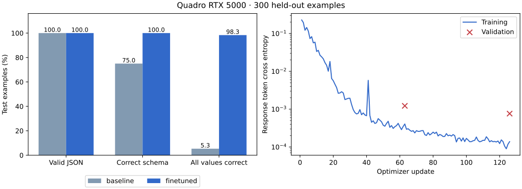
Each saved preview records the customer message, expected JSON, raw generated response, current update, epoch, and training loss. It checks JSON validity, schema compliance, and whether all values match. The checks distinguish invalid JSON from valid objects with incorrect fields or values. This matters because our recorded baseline already produced valid JSON on every test example, while getting all values right on only 5.33% of them.
The displayed loss comes from the training batch just processed. The generated response comes from a validation example after that update, so the two describe different checks. One optimizer update normally combines eight microbatches of four training examples. The preview adds one generation call after those 32 examples.
Generation, scoring, saving, and displaying a preview take extra time. We record that time separately from the training loop and save each sample immediately in previews.jsonl; completed runs also include them in training.json. We inspect saved samples locally. Keep previews off for the performance comparison: even with separate timers, generation can affect GPU memory and timing.
Keep the first configuration small
The full experiment uses these settings:
| Setting | Value |
|---|---|
| Model | Qwen2.5-0.5B-Instruct, pinned revision |
| Training / validation / test examples | 2,000 / 200 / 300 |
| Epochs | 2 |
| LoRA rank / alpha | 8 / 16 |
| LoRA targets | Query and value projections |
| Learning rate | 0.0002 |
| Optimizer | AdamW |
| Microbatch | 4 |
| Gradient accumulation | 8 |
| Effective batch | 32 |
| Padded sequence length | 256 tokens |
| Precision | FP16 mixed precision, FP32 adapter weights |
A microbatch is the group processed by one forward and backward pass. Gradient accumulation lets us process eight groups of four before making one optimizer update. That gives us an effective batch of 32 without holding all 32 examples’ activations in memory at once. The final group of an epoch can be smaller.
Response lengths vary. We normalize each microbatch’s contribution by its share of the response tokens in the entire accumulation window. This makes the accumulated gradient match a mean loss over those tokens rather than an average of differently sized groups.
We use the same FP16 configuration on both GPUs for the main comparison. Gradient scaling helps preserve small gradients, while the trainable adapter weights remain in FP32. Skipped optimizer updates are recorded so numerical failures cannot quietly appear as successful fast training.
Three separate workflows
The files are in blog/src/content/drafts/teaching-a-small-llm-to-output-json-with-lora/experiment/.
| Workflow | Entry point | Where training runs |
|---|---|---|
| Local GPU | run_local.py | The local NVIDIA GPU |
| Molab notebook | molab_notebook.py | The GPU attached to molab |
| Tinker | run_tinker.py | Tinker’s managed training service |
Both GPU paths use Python 3.12.13 and the same pyproject.toml and uv.lock, including PyTorch 2.7.1 with CUDA 12.8. PyTorch introduced official Blackwell support in its 2.7 release. The runner verifies actual versions before loading the model and records the lock hash in each manifest. GPU drivers remain specific to each host.
Run on the local GPU
From the experiment directory:
uv sync --locked
uv run run_local.py train --smoke --label local-smoke
uv run run_local.py train --label quadro-rtx5000
Start with the --smoke command. It uses 100 training examples, 20 validation examples, 24 test examples, and one epoch. It checks the complete path through tokenization, CUDA, gradients, saving an adapter, and generating responses. Its scores are a setup check rather than a substitute for the full experiment. The command without that flag runs the full experiment.
Each run saves its exact dataset, model revision, package versions, configuration, and raw predictions. Local runs also save the adapter weights. Unique output directories keep a later run from replacing an earlier measurement.
Run on molab
For molab, use experiment/molab_notebook.py. This is a minimal, single-file runner with five helper modules and the shared environment lock bundled inside. It provides GPU information, run settings, training progress and a results download. Analysis stays on the local machine. You do not need to import a Jupyter .ipynb file or upload the helper files separately.
Use the version marked MOLAB GPU NOTEBOOK V7. The notebook interface can run on molab’s Python 3.13 while training runs in a separate Python 3.12.13 process. That process uses uv’s locked project environment with the same dependency lock as the local runner; it does not use the notebook kernel’s preinstalled PyTorch. Its first launch may download the interpreter and packages. This is necessary because our first molab smoke run used different package versions despite the inline metadata. If the package manager offers to install data, engine, or runtime, import V7 into a fresh notebook; those are bundled helper names.
Import that Python notebook into molab, then enable the GPU using the notebook specs control in the header. Molab offers an RTX PRO 6000 Blackwell GPU. Check the notebook’s hardware information before training: it should show the attached GPU and CUDA-enabled PyTorch.
Select and click the large button inside the notebook. The toolbar play button executes setup cells; training waits for this button. After the smoke run succeeds, select and click it again. Training cells use marimo’s explicit execution controls.
Live generation previews are disabled in the molab notebook. It shows training status and saves losses and predictions for local analysis.
The notebook runs on its attached GPU and saves the baseline evaluation, LoRA training history, adapted evaluation, and adapter weights. It contains no reference runs, charts, saved-run selectors, benchmark sweeps, or Tinker controls. We compare the downloaded Blackwell run with the saved Quadro run locally.
When training finishes, a button appears automatically. Download that run before ending the session, then bring the ZIP here for analysis. It contains the predictions, training statistics, configuration, datasets, and adapter weights under artifacts/RUN/. Download the smoke and full run separately if you want both. Molab treats ordinary program-generated files as temporary storage, so saving the notebook alone does not preserve all experiment artifacts.
Measurements on the Quadro RTX 5000
The first full run used the configuration above and evaluated every held-out request without repairing the responses:
| On 300 held-out requests | Original model | After LoRA training |
|---|---|---|
| Valid JSON | 100.0% | 100.0% |
| Correct schema | 75.0% | 100.0% |
| All values correct | 5.3% | 98.3% |
The Quadro RTX 5000 completed 126 optimizer updates in 8.89 minutes of training time, processing 997 non-padding input tokens per second. Peak allocated GPU memory was 3.82 GiB. There were 0 skipped updates.
Here is one request the original model failed:
My request for order 28956 is to return 8 keyboards, please.
{"action": "return", "order_id": 28956, "product": "", "quantity": 8}{"action": "return", "order_id": 28956, "product": "keyboard", "quantity": 8}The raw scores, predictions, configuration, and loss history are saved in results/quadro-rtx5000.json beside this article. The figure is generated from that file’s source run. These are observations from one seed on this synthetic task; a high score here does not establish reliability on arbitrary requests.
All five remaining errors come from one held-out wording template: “There are … in order …; could someone … them?” Four have quantity 1, where the template produces awkward agreement such as “There are 1 mouse.” The other error swaps the order ID and quantity. This gives us a concrete follow-up: correct the generator’s agreement and add a separately written test set. We keep this first run and its dataset frozen so the hardware comparison uses the same workload.
First smoke run on Blackwell
The first returned molab run completed on an NVIDIA RTX PRO 6000 Blackwell Server Edition. It used the smoke configuration: 100 training examples, 20 validation examples, 24 test examples, and one epoch. That gave us four optimizer updates, with none skipped. Its raw results are saved in results/blackwell-smoke.json.
| Check on the 24 test requests | Before training | After training |
|---|---|---|
| Valid JSON | 24/24 (100%) | 24/24 (100%) |
| Correct schema | 17/24 (70.83%) | 23/24 (95.83%) |
| All four values correct | 0/24 (0%) | 5/24 (20.83%) |
Product extraction improved from 0 to 9 correct values out of 24, and quantity extraction improved from 16 to 21. Missing order IDs remained a problem: after training, the model invented an ID for seven of the eight requests without one. These are observations after only four updates; the full experiment is the next measurement.
The training loop took 1.51 seconds, while the four live previews added 1.49 seconds. These exclude model loading, baseline and final generation evaluation, and validation. Peak allocated GPU memory was 3.82 GiB, including validation and previews. Training loss went from 0.244 on the first update to 0.167 on the last, with an increase on update 3. The last live preview still returned an empty product and quantity zero for a request to cancel eight mice, despite producing valid JSON with the correct types.
This smoke run cannot supply a controlled speedup against the earlier full Quadro run. Besides the different workload and enabled previews, the saved manifest records PyTorch 2.11.0 with CUDA 13.0 on molab, while the Quadro used PyTorch 2.7.1 with CUDA 12.8. The actual recorded environment differs from the notebook’s dependency metadata. We need full runs with matching workloads and aligned software versions before interpreting a timing ratio.
Starting with V6, the runner addresses this by launching training with the shared lock and verifying the worker’s Python, package versions, and CUDA build. V7 retains that environment and always disables previews. The original smoke result remains unchanged. Code fingerprints normalize the relative imports used by bundled helpers, so packaging alone does not create a false difference.
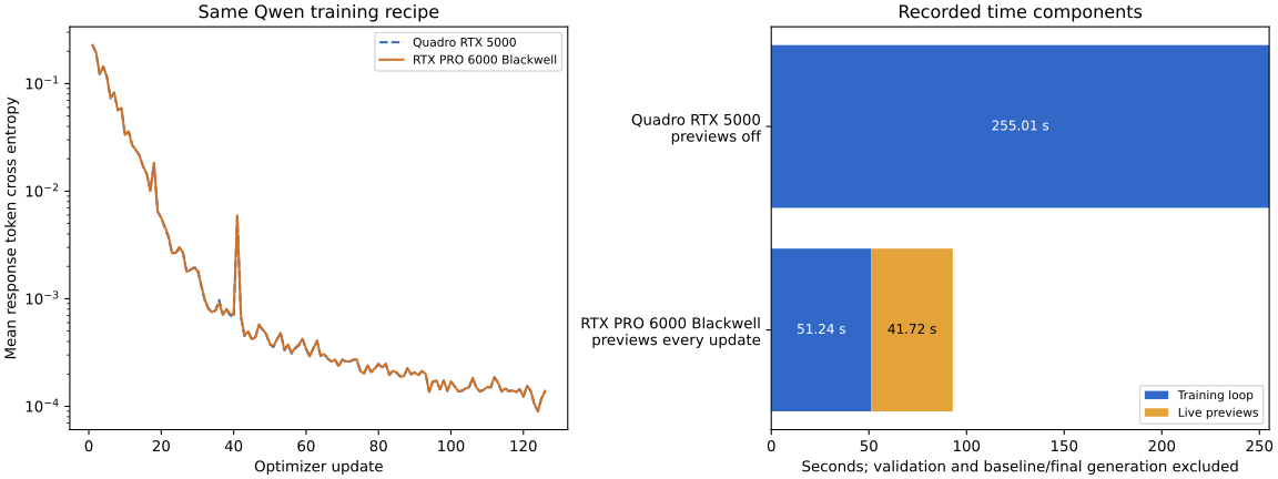
The fresh Quadro counterpart completed 126 updates in 255.01 seconds, with previews off and no skipped updates. It again reached 295/300 exact matches, and its training and validation loss history was identical to the first Quadro run. Its dataset, code, and environment fingerprints are saved in results/quadro-aligned.json. This is the local reference for the V6 Blackwell comparison below. The earlier run’s 533.10-second timing remains preserved; these two observations on the same GPU also show why timing ratios need fresh runs and repeated measurements rather than an assumption that one recorded duration is fixed.
Full Qwen run on Blackwell
The returned V6 run used the full dataset and passed the alignment checks: Python 3.12.13, PyTorch 2.7.1 with CUDA 12.8, package versions, model revision, dataset, code hash, environment lock, precision, and batch configuration match the fresh Quadro run. The saved results are in results/blackwell-full.json.
| Recorded measurement | Quadro RTX 5000 | RTX PRO 6000 Blackwell |
|---|---|---|
| Optimizer updates | 126 | 126 |
| Training loop | 255.01 s | 51.24 s |
| Live preview overhead | 0 s | 41.72 s |
| Non-padding input tokens per second | 2,085 | 10,375 |
| Peak allocated GPU memory | 3.82 GiB | 3.82 GiB |
| Exact matches after training | 295/300 | 295/300 |
Both runs produced valid JSON and correct schemas on all 300 test requests after training. All 300 final raw responses were identical between the GPUs, including the same five mistakes. Their training losses differ slightly, as can happen with different GPU kernels and FP16 arithmetic, while the generated test answers agree.
One monitoring setting differs: the Blackwell run generated a preview after every update, while the Quadro had previews off. The recorded training-loop time ratio is 4.98×, excluding those previews. This is an observed component ratio rather than a fully matched GPU benchmark; generation between updates can affect GPU state and scheduling even when timed separately. The Blackwell previews alone added 41.72 seconds to its 51.24-second training loop. For the timing rerun, import V7, select , and click . V7 always disables previews.
Authenticated Tinker training remains pending and will be reported as a separate service workflow.
Compare the two GPUs
First run the identical full experiment on each machine. Keep the model, dataset, sequence length, precision, microbatch, gradient accumulation, and software versions fixed. Extract the downloaded molab run beside the local run and compare these settings and fingerprints in their manifest.json files before interpreting timing ratios. The local reporting.py helper flags differences when comparing runs.
Training time covers the training loop, including transfers, forward and backward passes, and optimizer updates. Downloads, model loading, generation evaluation, validation, and live previews are outside that timer. Preview overhead is recorded separately. The initial training update is included. Report peak allocated GPU memory and non-padding input tokens per second alongside the elapsed time. Peak memory includes validation and previews when enabled, so disable previews on both hosts for the controlled comparison.
Input tokens include both prompts and responses because both take computation. Only response tokens contribute directly to the loss. The sequences are padded to 256 tokens on both GPUs; padding does not inflate the throughput numerator.
Then run a separate batch-size sweep:
# On the Quadro machine
uv run --locked run_local.py sweep --microbatches 4 8 16 --output artifacts/sweep-quadro.json

# On the Blackwell machine
uv run --locked run_local.py sweep --microbatches 4 8 16 32 --output artifacts/sweep-blackwell.json
Compare microbatches 4, 8, and 16 on both machines, and also try 32 on Blackwell, adjusting accumulation to keep 32 examples per update. Each trial restores the same adapter initialization and resets the optimizer. It performs three warmup updates, times ten updates, and repeats the measurement three times. We plot median throughput against microbatch size. An out-of-memory result ends the sweep.
On molab, import the separate experiment/molab_sweep.py notebook, enable the GPU, click , and save when it finishes. It runs microbatches 4, 8, 16, and 32 using the shared locked benchmark implementation. The training notebook remains unchanged, and all analysis stays local. Run only one GPU experiment at a time.
Increasing the microbatch usually increases activation memory: more examples are processed together, while the model weights remain the same size. With effective batch 32, microbatch 4 takes eight forward/backward passes per optimizer update; microbatch 32 takes one. More GPU memory lets us try those larger microbatches. Filling memory alone is not a performance objective, and the 3.82 GiB used by our original run does not measure compute utilization.
This answers two different performance questions: how quickly each machine runs our fixed training recipe, and how throughput changes when we give the GPU more work per pass. A small model can leave a powerful GPU waiting on host work or small operations, so its speedup need not resemble a ratio of advertised compute figures. The hypothesis for this sweep was that the gap would grow with microbatch size; the results below show how much it changed.
As GPU computation gets faster, CPU dispatch, data movement, and synchronization can become a larger fraction of elapsed time. The main training loop reads a finite-loss check and a scalar loss back to Python after each microbatch. Such reads introduce synchronization; PyTorch recommends minimizing them. The sweep omits these per-microbatch diagnostics, so compare sweep settings with each other rather than treating their timings as repetitions of the full training run. A profiler is still needed to establish which costs dominate.
Inference needs another control. Copy the same saved adapter onto both machines before timing it. Otherwise, different trained weights may generate different responses, making a latency comparison harder to interpret. The inference runner records adapter and prompt hashes, generated token counts, median request latency, and aggregate output tokens per second at batch size 1.
These are whole-machine measurements. CPU performance, GPU power limits, clocks, library dispatch, and competing jobs can affect the result. A hardware change should mainly change time, although floating-point differences mean the trained weights and greedy outputs need not be identical.
What the Quadro sweep showed
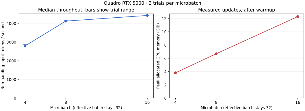
The completed repeat kept 32 examples per optimizer update and measured three trials at each setting. No optimizer updates were skipped:
| Microbatch | Accumulation steps | Median input tokens/s | Speed relative to microbatch 4 | Peak allocated memory |
|---|---|---|---|---|
| 4 | 8 | 2,794 | 1.00× | 3.82 GiB |
| 8 | 4 | 4,123 | 1.48× | 6.69 GiB |
| 16 | 2 | 4,425 | 1.58× | 12.29 GiB |
Increasing the microbatch helped, but throughput began to flatten. Doubling it from 8 to 16 increased throughput by only 7.3%, while peak allocated memory rose from 6.69 to 12.29 GiB. More occupied memory did not produce a proportional speedup. This measures the whole loop and does not establish whether computation, memory traffic, or host overhead sets the remaining limit.
The first attempt exposed a measurement problem: the Quadro’s reported power limit changed from 50 W to 110 W during the sweep, and its clocks increased sharply. Microbatch 16’s recorded rates ranged from about 917 to 4,734 tokens/s. Microbatch 32 then occupied nearly all reported device VRAM and completed one slow trial at about 626 tokens/s; we interrupted the remaining trials. There was no recorded out-of-memory exception. We preserve that attempt as an interrupted diagnostic, not a batch-size comparison.
The table uses a fresh sweep of 4, 8, and 16 after that transition. Sampled GPU power-limit reports were 110 W during the repeat; power draw and clock rates still varied. Raw trial timings and memory allocations are in results/sweep-quadro.json, with the diagnostic attempt and telemetry preserved under experiment/artifacts/. These sweep timings should not be substituted for the earlier full-training timing.
How Blackwell scaled with microbatch size
The returned Blackwell sweep matches the Quadro’s model revision, dataset, code hash, configuration, package versions, environment lock, warmup, measured updates, and repetition count. Each measured trial processed the same 42,630 non-padding input tokens. All twelve Blackwell trials completed with no skipped optimizer updates recorded in their measured intervals.
| Microbatch | Quadro input tokens/s | Blackwell input tokens/s | Blackwell speedup at the same microbatch | Peak allocated memory |
|---|---|---|---|---|
| 4 | 2,794 | 11,478 | 4.11× | 3.82 GiB on each |
| 8 | 4,123 | 19,133 | 4.64× | 6.69 GiB on each |
| 16 | 4,425 | 21,619 | 4.89× | 12.29 GiB on each |
| 32 | No completed three-trial result | 25,116 | — | 23.60 GiB on Blackwell |
Blackwell’s throughput increased 2.19× between microbatches 4 and 32. At the shared settings of 4 and 16, it improved 1.88×, compared with 1.58× on the Quadro. Its lead at the same microbatch grew from 4.11× to 4.89×. Larger batches helped Blackwell more, and its lead at matched settings grew by about 19%.
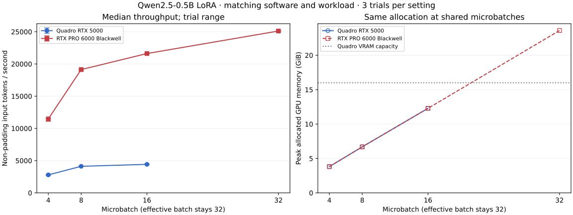
The memory measurements make the capacity distinction concrete. Both GPUs allocated exactly the same peak number of bytes at each shared setting. Blackwell’s extra memory gave us room to complete microbatch 32, whose 23.60 GiB allocation exceeds the Quadro’s roughly 16 GiB of VRAM. Comparing the best completed settings, Blackwell at 32 was 5.68× faster than Quadro at 16; that is a comparison using different microbatches, separate from the matched-setting ratios in the table.
These results show batch-size scaling, not a breakdown of the remaining costs. They do not prove that CPU dispatch or synchronization dominates, or that either GPU has reached its maximum throughput. A profiler would be needed for that diagnosis. The hosts still differ in CPU, driver, and power budget: the Quadro used six PyTorch CPU threads, Blackwell used twenty, and Blackwell reported a 600 W power limit. Trials timed only ten optimizer updates after three warmup updates; repeat sessions would help assess longer-term variability.
The complete Blackwell measurements are saved in results/sweep-blackwell.json, and the matched-setting ratios are in results/sweep-comparison.json. The training notebook and its fixed-recipe results remain separate from this throughput experiment.
Teach a smaller model the output format
Qwen’s JSON validity is already at the ceiling on our measured requests. Its model card specifically highlights structured output and JSON capabilities. The extraction improvement is useful, but a model that already follows the format cannot show us much improvement in that metric.
For the second experiment, we use SmolLM2-135M-Instruct. An exploratory probe on the first 20 validation requests produced no valid JSON responses. Nine generations hit the 96-token limit; the eleven that finished were also invalid as complete JSON responses. The model often repeated the customer message or wrapped an answer in prose and Markdown. We saved that probe in results/smollm2-135m-probe.json and kept the final test set untouched until the full experiment.
The separate runner uses a pinned model revision and the same 2,000 training, 200 validation, and 300 test examples as Qwen. It reuses the LoRA training and scoring implementation, with two epochs and rank 8 on query and value projections. For this model, 460,800 adapter parameters are trainable. Run it locally with:
uv run --locked python formatting/run.pyThe complete run gave us this before-and-after result on the same 300 held-out requests:
| Check | Before fine-tuning | After fine-tuning |
|---|---|---|
| Valid JSON | 0/300 (0%) | 300/300 (100%) |
| Correct schema | 0/300 (0%) | 300/300 (100%) |
| All values correct | 0/300 (0%) | 207/300 (69%) |
| Responses reaching the token limit | 179/300 | 0/300 |
These formatting failures concern the complete response. They include explanations, Markdown fences, repeated answers, and incomplete generations; they do not imply that every response had a misplaced comma. Even the 121 baseline responses that finished before the token limit failed an ordinary JSON parse. After training, every test response was a complete JSON object with the required schema.
Here is one request whose values and output format improved:
Items: 3 monitors. Order reference: order 24179. What I need: track.
You need to track a specific order. The order reference is "order 24179", and the order ID is 3.{"action": "track", "order_id": 24179, "product": "monitor", "quantity": 3}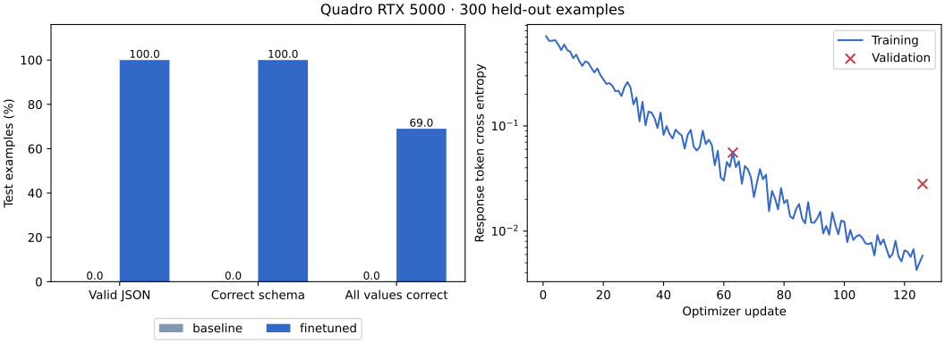
The live previews show the distinction as learning progresses. The sample at update 10 still contained prose and Markdown. At update 20, a sample passed the JSON and schema checks but used the order number as its quantity. At update 50, a sample matched every field. These are different validation requests, so the final test scores provide the aggregate comparison.
Training took 290.26 seconds for 126 updates, with no skipped updates. Thirteen previews added 44.00 seconds, and peak allocated GPU memory was 1.47 GiB. The raw predictions, configuration, losses, previews, and model revision are saved in results/smollm2-formatting.json; the trained adapter remains in the formatting run’s artifact directory.
The remaining errors include copying an order ID into the quantity, inventing an absent ID, and changing quoted product names. One held-out wording template, “There are …; could someone …?”, accounts for 51 errors among its 70 requests. Formatting is now reliable on these examples, while extracting the values still needs work. Size, architecture, and prior training all differ from Qwen, so this does not isolate parameter count as the cause. We keep the Qwen hardware workload fixed and report SmolLM2 as a separate formatting experiment.
Run the same task through Tinker
Tinker lets us write the data preparation and training loop locally while a managed service performs the training computation. We send token sequences and loss inputs through the SDK, then request samples from the resulting checkpoint.
Its current model catalog does not list Qwen2.5-0.5B-Instruct. Our Tinker path therefore defaults to Qwen3.5-4B, with thinking disabled. The dataset and quality checks stay the same. Model size, adapter layout, precision, and infrastructure differ, so we report it as a separate workflow comparison rather than a third GPU speed measurement.
Install the optional SDK, authenticate, and check the available models:
uvx --from tinker==0.33.1 tinker auth login
uv run --script run_tinker.py --list-models
uv run --script run_tinker.py --dry-run --smoke
Tinker uses its own run_tinker.py script and client environment, without loading the CUDA engine or marimo. The dry run checks the selected tokenizer, masks, sequence lengths, and SDK data objects without calling the Tinker service. To train, run:
uv run --script run_tinker.py --smoke
uv run --script run_tinker.py
Those training commands use your service account for training and sampling. Keep credentials in Tinker’s login storage or the TINKER_API_KEY environment variable.
The SDK’s cross entropy loss sums weighted token losses. Our runner assigns zero weight to prompt tokens and normalizes response weights over the full batch. Unlike the local Hugging Face call, Tinker’s data objects receive explicitly shifted input and target sequences.
Tinker results include baseline and adapted quality scores, losses, client wall time, and checkpoint paths. Awaiting each operation includes network and queueing in that time. Actual service charges belong beside those observations when available from the account’s billing view. They cannot be inferred from a GPU rental rate.
What to learn from the results
Read validity, schema compliance, and exact accuracy together. If JSON validity is already high, training may still improve the consistency of fields and values. If training loss falls while held-out accuracy stalls, inspect the failures before adding more epochs.
Look separately at missing order IDs, plural products, and names containing quoted words. Those examples reveal different mistakes: inventing an ID, failing to normalize a product, or escaping its name incorrectly. Each run saves all raw responses so we can inspect those patterns locally.
Supervised fine-tuning makes the desired response more likely. It does not guarantee a valid response on every future input. A useful next experiment is constrained decoding, which restricts the allowed tokens according to a grammar or schema. It can enforce supported structural rules, while the values still need checking against the request.
For this first experiment, the useful outcome is a clear before-and-after measurement, a set of understandable failures, and a reproducible workload we can move between machines.
For the hardware comparison, roughly 5× faster on Blackwell is a reasonable expectation for this Qwen model, FP16 LoRA setup, and training implementation. The sweep measured 4.1–4.9× at matching microbatches. Comparing each machine’s best completed setting gave about 5.7×, with Blackwell at microbatch 32 and Quadro at 16. These are whole-machine results for this workload. Larger models, longer sequences, or different implementations could produce a different gap.