What compression preserves in a neural network
In Directions, sparse features, and how sparse autoencoders find them, we explored how several feature directions can share an activation space, and how sparsity can help us recover their contributions. Here we’ll train a network on a different problem: predicting a price from three continuously varying house attributes, with only two hidden coordinates.
But affecting a representation and being recoverable from it are different things. Can we read all three attributes back out? Which distinctions disappear? And does a direction with very little variation still carry useful information?
We’ll freeze the trained weights and investigate those questions with singular value decomposition (SVD), linear probes, and controlled interventions. We’ll distinguish prediction accuracy, variation in hidden space, and recoverability of the original features. We’ll also compare trained representations against their random initializations: recoverability after training does not, by itself, establish that training discovered a feature.
A price formula whose answer we know
We’ll use size, rooms, and age as names for three independent synthetic feature scores:
Each score is sampled uniformly from , giving population mean zero and variance one. These are continuous standardized scores: “rooms” is not an integer room count, and is a price score rather than dollars. The coefficients are chosen for the experiment, not estimated from a housing market.
Using comparable scales keeps a large physical unit from dominating the geometry. Sampling independently also prevents a probe from recovering age merely because older houses happen to be smaller. Real housing data would introduce both complications.
The model computes:
with matrix shapes , , and . Our main experiment uses ; controls use and .
All layers are linear and have no biases. The target has zero intercept, so biases are unnecessary. We supply the input attributes directly, but give the model no labels or auxiliary losses telling it what its hidden neurons should mean. This experiment studies learned representations of known inputs; it does not discover house attributes from raw images or text.
Training uses the familiar loop: forward pass, mean squared error, backpropagation, and gradient descent. Here is the complete parameter update, with examples stored as rows:
h1 = X @ W1.T
h2 = h1 @ W2.T
error = h2 @ W3.T - y       # y has shape (N, 1)
delta = 2 * error / len(X)

grad_W3 = delta.T @ h2
grad_W2 = (delta @ W3).T @ h1
grad_W1 = (delta @ W3 @ W2).T @ X

# Compute every gradient before changing any weight.
W1 -= 0.03 * grad_W1
W2 -= 0.03 * grad_W2
W3 -= 0.03 * grad_W3
We use 2,048 training examples and 4,096 held-out examples, with a fixed data seed. For each width, we train five initializations: seeds 7, 11, 23, 42, and 101. Initial weights are independent normal samples with standard deviation 0.4. Training stops when training MSE is below , with a maximum of 10,000 updates. Every run converged in 123–214 updates.
The PCA bases and probes are fitted on training activations only. Reported correlations, probe scores, and prediction errors use the held-out examples. These runs characterize this setup; five seeds are not a statistical survey of all possible training choices.
One dimension is already enough to predict price
Because the layers are linear, their composition is linear:
The target depends on just one scalar combination, . A one-neuron bottleneck could store that number and let the final layer return it. Predicting price accurately therefore does not require retaining the three inputs separately.
All 15 trained networks reached held-out price MSE below . This is an easy, exactly representable task; those tiny errors are numerical agreement, not evidence of realistic house-price forecasting.
The useful question is what else survived on the way to that answer.
These are trained weights. Move an input, inspect its hidden point, then move along the lost direction.
Axes scale independently to expose the thin second dimension. Displayed angles and aspect ratio are not the hidden space’s geometry. PC variance shares: 99.905% / 0.095%.
n = [-0.2971, 0.7197, 0.6275]. Changing t changes the features, but the hidden point and predicted price stay fixed.
| Feature | Original x | Changed x′ | Probe estimate from h₂ | Test R² |
|---|---|---|---|---|
| Size | 0.4000 | 0.4000 | 0.3677 | 0.914 |
| Rooms | -0.2000 | -0.2000 | -0.1218 | 0.499 |
| Age | 0.3000 | 0.3000 | 0.3682 | 0.615 |
Five runs, the same training and test data. Seed 7: test price MSE 9.87e-21. Feature scores are synthetic, continuous, and standardized; “rooms” is not an integer room count.
Start by moving size while leaving rooms and age fixed. The white point follows a line in the two-dimensional bottleneck. Now move rooms: another input change also moves that same point. Switch seeds and notice that accurate prediction survives changes to the internal representation.
Three neurons can preserve three features without naming them
In our main run, seed 7, the first hidden layer learned approximately:
Each row describes one neuron. The first neuron responds to all three attributes; it is not a dedicated size coordinate. The other rows are mixtures too.
Nevertheless, this matrix has rank three. Its transformation is invertible, so the full hidden vector contains enough information to recover all three inputs. We verify this with separate linear readouts fitted after freezing the network.
The first layer retained rank three in all 15 runs. That is an observation, not something the price loss requires. The random initial first layers were already full rank, so full recoverability here is not evidence that training discovered three concepts. Training changed a representation that already had enough capacity to preserve the input.
For an example where the known properties are combinations of raw inputs, see the related experiment on brightness and contrast in a two-pixel autoencoder.
Three feature directions share two dimensions
Combine the first two layers into . Then . For seed 7:
The three columns describe how changing each input changes the hidden vector:
The hidden vector is the sum of their contributions:
All three columns are nonzero: all three features affect the representation. The network represents three input features using directions in a two-dimensional space. Each feature can affect the representation, but their effects cannot all be distinguished independently.
This is what sharing representational space means in our experiment. The three feature arrows need not point in exactly the same direction. But they cannot all be linearly independent: at least one is a combination of the others. A change in one feature can therefore be canceled by changes in the other features, leaving the same hidden vector. Observing an effect of every feature does not establish that we can read every feature back out.
We’ll make that ambiguity concrete by finding the combination of input changes that the bottleneck loses.
Since has rank two, there is a nonzero input direction with . SVD of the weight map finds it:
_, _, Vt = np.linalg.svd(B, full_matrices=True)
n = Vt[-1]  # Third right singular vector, in the 3D INPUT space.
full_matrices=True matters here: a reduced SVD of this matrix returns only two right singular vectors and omits the null direction. SVD signs are arbitrary; we choose the sign making the largest-magnitude entry positive.
Our lost direction is approximately:
Now compare two inputs and :
The network cannot distinguish a slightly smaller house with more rooms and greater age from the original when those changes follow these proportions. For interior points, small changes along remain inside our sampled input domain, so this is a real ambiguity within the experiment.
Move the widget’s lost direction slider. The input attributes change while the hidden point and prediction stay fixed. The true price also stays fixed to training precision: the learned null direction is almost perpendicular to .
No decoder, linear or nonlinear, can recover every original input from identical hidden vectors. The information has been discarded. SVD cannot restore it.
SVD of activations answers a different question
Now collect bottleneck activations for the training examples into . Center them and compute:
This time the right singular vectors live in the two-dimensional hidden space. They give principal component directions: perpendicular axes ordered by the activation variance along them.
mean = H_train.mean(axis=0)
_, singular_values, Vt = np.linalg.svd(H_train - mean, full_matrices=False)
scores_test = (H_test - mean) @ Vt.T
variance_share = singular_values**2 / np.sum(singular_values**2)
NumPy’s SVD documentation describes the returned factors. For these real matrices, the rows of Vt are the axes onto which we project.
In seed 7, the bottleneck’s singular values are approximately 79.249 and 2.446. PC 1 accounts for 99.905% of training activation variance; PC 2 accounts for 0.095%. The cloud is almost a line, but its second dimension is not zero.
We know the feature labels, so we can measure correlations between held-out PCA scores and each feature:
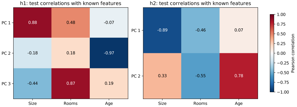
For the bottleneck:
| Component | Size correlation | Rooms correlation | Age correlation |
|---|---|---|---|
| PC 1 | −0.890 | −0.457 | 0.072 |
| PC 2 | 0.334 | −0.547 | 0.783 |
The first component is strongly associated with size, but also with rooms. The second is strongly associated with age, but is still a mixture. SVD supplied statistical axes; the labels let us investigate their meaning afterward.
Notice how much age association sits in a component explaining less than one tenth of one percent of hidden variance. A rule that retained only enough components to explain 99% of variance would drop it. Small variance does not imply irrelevant information, although a small signal can be less robust to noise. Our current measurements have no added activation noise.
A probe measures what the whole representation can recover
Correlating one PCA coordinate with age asks about that coordinate alone. To use all available coordinates, fit a separate linear regression from frozen activations back to the inputs:
This is a linear regression probe. The network remains frozen; feature labels supervise only the diagnostic readout. Alain and Bengio’s work on linear classifier probes uses the same separation between a trained representation and independently trained diagnostic classifiers. Here our targets are continuous.
design = np.column_stack((H_train, np.ones(len(H_train))))
probe = np.linalg.lstsq(design, X_train, rcond=None)[0]
recovered = np.column_stack((H_test, np.ones(len(H_test)))) @ probe
We report held-out : 1 means exact recovery; 0 corresponds to the error of predicting the held-out feature mean. Scores can be negative. These are predictive scores, not percentages of information or proof that the original model uses a feature in a particular way.
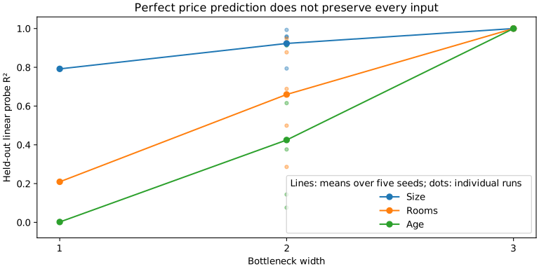
| Bottleneck width, seed 7 | Size R² | Rooms R² | Age R² | Price R² |
|---|---|---|---|---|
| 1 | 0.792 | 0.209 | 0.002 | ≈1 |
| 2 | 0.914 | 0.499 | 0.615 | ≈1 |
| 3 | 1.000 | 1.000 | 1.000 | ≈1 |
The two-neuron representation partially predicts all three features while recovering none exactly. Mixing allows each feature to affect the representation, but leaves ambiguity about their separate values.
Across the five two-neuron runs, age R² ranges from 0.076 to 0.913 despite equally accurate price predictions. The extra direction retained beyond price depends on initialization and training; it is not uniquely specified by the target.
There is also an exact population check. Our inputs have covariance , so the optimal linear reconstruction from is its projection onto the row space of . If , where is the pseudoinverse, then:
These are population optimal linear-probe scores. The finite training and test estimates above need not sum exactly to the rank. This identity is specific to our isotropic inputs and this linear recovery criterion; it is not a general law for neural representations.
Change the geometry without changing predictions
The price loss does not uniquely determine hidden coordinates. Take any invertible matrix and replace:
Then for every input. An invertible change preserves the information available to a refitted linear probe, but a nonorthogonal change can alter angles, lengths, and PCA variance shares.
The experiment applies:
For seed 7, the first component’s variance share changes from about 99.905% to 99.980%. Predictions and probe R² stay unchanged within numerical tolerance. Toggle Change hidden basis; preserve predictions to inspect this transformation. It re-expresses the frozen network; it does not retrain it.
This proves nonuniqueness directly. Separate training runs need not be related by this exact transformation: they may also retain different input subspaces, as our varying probe scores demonstrate.
Change a hidden direction and check its effect
Because we control the inputs, we can identify an exact hidden intervention corresponding to increasing one feature. Holding the original input fixed, add to its bottleneck activation:
The script tests these interventions on the held-out examples. For , adding the size direction changes predicted price by 0.50; the rooms direction changes it by 0.25; the age direction changes it by −0.05.
These are writing directions: they describe how an input change enters hidden space. A probe is a reading direction: it tries to infer an input value from the activation. They need not coincide. Here there cannot be perfect independent readouts for all three features, since their writing directions are dependent.
The intervention verifies a mechanism for this model’s scalar output. It does not establish that a hidden axis represents an abstract concept such as “desirability.” We would need a definition and independent measurements to test that interpretation.
Is this superposition?
In interpretability research, superposition means representing more features than there are dimensions, using overlapping feature directions. Toy Models of Superposition investigates this with sparse input features and small ReLU networks, including how nonlinear filtering handles interference.
Our experiment has the associated geometry: three feature contributions share two hidden dimensions, and changes in those contributions can cancel each other. But the training objective only rewards preserving one price combination. It gives the model no obligation to keep size, rooms, and age separately recoverable. Accurate price prediction therefore does not establish that the network learned to preserve three distinct, independently useful features in superposition.
This experiment illustrates the overlapping feature directions underlying superposition. However, because training rewards only price prediction, it does not establish that the network learned to preserve all three features as separately recoverable quantities.
Imperfect recovery alone does not rule out superposition: interference and reconstruction errors can be part of it. Nor does the definition require ReLU. The limitation of our evidence is that we have not tested an objective that rewards retaining the individual features.
A stronger follow-up would train the two-neuron bottleneck to reconstruct all three inputs, introduce sparse feature activity so that features are often zero, and compare linear and nonlinear decoders. We could then measure which features remain recoverable and how often their overlap causes errors. Preserving several features would become something training explicitly rewards, allowing us to investigate when sharing dimensions helps that task.
What this tells us about LLM vector spaces
This tiny network gives us a controlled way to distinguish coordinates, feature directions, statistical components, and information lost by compression. Those distinctions are useful when approaching larger models: a correlated activation is not automatically a unique concept, and successful prediction does not uniquely specify an internal representation.
It does not establish how a particular language model represents concepts. Our inputs have known meanings, the transformations are globally linear, and we can generate matched examples by changing one variable. Language-model analysis must establish which of those assumptions, if any, is reasonable for the representation being studied.
Another follow-up would add a nonlinear price target, such as a bonus when size and rooms both exceed thresholds, and compare the linear model against a ReLU network. That would test whether nonlinear intermediate computations improve prediction. Merely inserting ReLU while keeping this linear target would not require the network to discover useful nonlinear features.
Reproduce and inspect every measurement
Download the NumPy experiment and the complete measured results. The JSON includes all 15 runs, weights, singular values, probes, correlations, null directions, and training histories. The widget evaluates those frozen weights in the browser.
python3 -m venv .venv
source .venv/bin/activate
python -m pip install numpy==2.2.6
python house_representation_experiment.py
Inside the repository, the first article’s directions-sparse-features-and-how-sparse-autoencoders-find-them/experiment/ directory also contains a README and pinned direct dependencies for regenerating the two SVG figures. Run python experiment.py --export --figures there after installing requirements.txt. Generated paths are relative to the script’s location, not the working directory; use the repository layout when regenerating the article assets.
The script checks backpropagation against finite differences, verifies the learned end-to-end formula, measures probes on held-out data, and checks nullspace invariance, hidden interventions, and prediction invariance under the changed basis. SVD signs and last-digit floating-point results may vary across numerical libraries.
The result is a concrete answer to our starting question. We can map learned mixtures back to known features to the extent that those features remain recoverable. SVD helps reveal how the representation varies; labels and controlled changes tell us what those variations correspond to. Neither can recover distinctions the network has erased.