Understanding ResNet: learned updates, transformer residual streams, and stability
https://chatgpt.com/c/6af387e0-ad90-83eb-9625-ae90bc9f0396
One of the key components of the transformer architecture is the residual connection. Its main job is to add the output of an attention or feed-forward sublayer to the token’s existing representation.
Residual connections go back to residual networks, or ResNets, which helped make very deep neural networks easier to train. Transformers use the same idea: instead of replacing a representation outright, each attention or feed-forward sublayer adds its output to its input.
In this article, we’ll explore how residual connections work, where they appear in a transformer, and why this simple addition matters.
The input follows two paths. The learned branch computes an update , while the skip connection carries directly to the addition:
Without the shortcut, the output would be . With it, the output is . In a transformer, the branch contains the attention or feed-forward computation, with normalization arranged according to the architecture. The addition itself has no learned weights.
“Residual architecture” describes this wiring around the addition. The input feeds both a learned branch and a direct shortcut, and the two paths meet at the sum. For a scalar example, suppose and the desired output is :
| Arrangement | What the learned branch must output for this input | Block output |
|---|---|---|
| Plain | ||
| Residual |
The shortcut already supplies , so the residual branch learns the required change. A residual block combines a path that carries the input, a branch that computes an update, and an addition that joins them. A residual network repeats this arrangement across many blocks.
One path carries the input unchanged; the other computes an update from it. Around an attention sublayer, the update branch uses learned query, key, and value projections, attention mixing, and an output projection. Around a feed-forward sublayer, it uses learned linear transformations and an activation function. In a pre-norm transformer, the normalization before the sublayer also belongs to the update branch. In each case, the direct path supplies the original input to the .
Both paths contribute to the output: the addition combines the original input with the computed update. Operations placed after the addition, such as post-norm layer normalization, then act on the combined result.
Residual connections helped make much deeper networks trainable by improving optimization. They also provide direct paths for gradients, helping reduce vanishing-gradient difficulties. The original ResNet work specifically addressed the degradation problem: adding layers could increase training error even when initialization and normalization had largely addressed vanishing or exploding gradients. We’ll examine that distinction below.
In a transformer, residual connections are the architectural mechanism; the residual stream is the running sequence of token representations they carry through the network. During the forward pass, each addition combines the current representation with a sublayer’s update. During backpropagation, the direct path contributes a gradient that does not pass through that sublayer’s computation.
Kaiming He, Xiangyu Zhang, Shaoqing Ren, and Jian Sun introduced ResNet in a December 2015 preprint, published at CVPR 2016. Their work demonstrated image networks up to 152 layers deep, and a residual-network ensemble won the 2015 ImageNet classification competition. Deep Residual Learning for Image Recognition established residual learning as a practical way to train much deeper networks.
Shortcuts had predecessors: Highway Networks, also from 2015, used learned gates to control information flow. In 2017, Attention Is All You Need, §3.1 explicitly adopted residual connections around its transformer sublayers and cited the ResNet work.
Why deeper networks sometimes trained worse
The original ResNet paper compared plain networks of different depths. On CIFAR-10, a 56-layer plain network had higher training error than a 20-layer one. A deeper plain ImageNet model showed a similar problem. This was called the degradation problem.
Higher training error distinguishes this observation from the usual overfitting story, where a model fits training data well but generalizes poorly. The authors also reported that initialization and normalization had largely addressed the vanishing/exploding-gradient obstacle in their setup. Additional depth still proved difficult to optimize.
Their motivating argument was to take a shallower model and insert extra identity mappings. If the added stages can represent identity while preserving the surrounding computation, the deeper model has a solution that reproduces the shallower model. Yet the tested training procedure did not reliably find a solution that good. Residual learning changed how those extra transformations were parameterized, and the paper demonstrated substantially improved optimization at greater depths.
The proposed shortcut carries a block’s input forward and adds a learned update to it. Before working with entire feature maps, let’s isolate that addition with just two numbers.
One block adds an update
Take the “patch” intuition literally as arithmetic:
The update increases one coordinate, decreases another, and leaves the third unchanged. “Patched” means element-wise addition. There is no replacement operation or requirement that the update affect only a few coordinates.
These numbers illustrate a possible branch output. During training, the branch receives no answer sheet listing the correct differences: its weights learn through backpropagation from the whole network’s loss.
To see how one update affects the next, use a two-dimensional example where we can draw every step.
Suppose the current representation is:
A residual block sends this vector along two paths. The shortcut carries it unchanged. The residual branch computes an update . The block adds the two results:
The branch can contain several neural-network layers. To make the arithmetic visible, we’ll choose a simple function by hand. Write the coordinates of its input as and define:
At , this branch reads the first coordinate and adds that amount to the second:
The branch’s output is , while the block’s output is . The shortcut makes the block output different from the output of its learned branch. In a CNN, we will apply this same addition to every position in every feature map.
The next block reads the updated vector
Let the second branch compute:
It receives , so it reads and produces :
| Block | Vector it reads | Update it computes | Vector after addition |
|---|---|---|---|
| First | |||
| Second |
Later blocks read the representation after earlier updates. The second branch does not independently read the original . Changing the first update can therefore change the second update too.
Use to follow both additions. The gray arrow shows the starting vector; orange and purple arrows show the updates added at each step. Then turn off and inspect what the second branch reads.
Both branches will read the current vector when their turn arrives.
With the first branch disabled, stays at . The second branch now computes instead of , giving a final vector of . Removing an early contribution changes the later computation; it is not generally equivalent to subtracting that early contribution from the original final answer.
A zero update preserves the input
If a branch produces zero, its residual block computes:
Disable both branches in the widget. The vector remains throughout. This is the identity mapping: the output equals the input.
For the same branch function in a plain block, the output would be . Setting would produce zero, rather than pass the input through. A residual block makes an unchanged output available by making its branch output zero.
This does not mean every residual block starts as identity or automatically learns to do nothing. Initialization, biases, normalization, and the branch’s parameters all affect its output. It also does not mean residual updates must be small: a branch can add a large change or cancel an existing value. For example, makes the sum zero.
Learn the change relative to the input
Suppose the desired block mapping is . We can express it as:
The word residual refers to this difference from the input. It is not necessarily the prediction error measured by the loss function.
Training still uses the final task loss. We do not normally supply a separate target for every internal block. Backpropagation adjusts the branch parameters through the addition so that the whole network performs its task.
When an identity mapping is useful, the branch only needs to produce zero. A parameter setting such as a zero final linear map with zero bias can make that possible. But gradient descent does not automatically zero every unhelpful branch, and weight decay is not a guarantee of identity behavior.
The shortcut gives a block an explicit path for the existing representation. The branch can learn a correction through its own layers. How much that helps training remains an empirical property of the architecture and training setup.
See what F learns: a correction to a blurry image
Image reconstruction makes the difference visible. Suppose is a blurry image and is the sharp image we want. Both have the same dimensions. A plain network must produce the desired image as its output. A residual model computes , so its branch should produce the correction .
The shortcut already carries the blurry house below. To sharpen it, the branch needs to increase brightness on one side of an edge and decrease it on the other. Areas that already match the target need no change. The middle panel shows those signed corrections explicitly:
| Pixel | Input | Correction | Result |
|---|---|---|---|
| Brighten an edge | 0.388 | +0.512 | 0.900 |
| Darken a window | 0.541 | -0.441 | 0.100 |
| Keep the background | 0.100 | 0.000 | 0.100 |
For each pixel, the addition is the same arithmetic as our vector example: existing brightness + correction = new brightness. The branch’s output can contain negative values even though the image brightness values are nonnegative. Simply adding positive values everywhere would brighten the image rather than restore its boundaries.
In a trained reconstruction model, the branch sees the blurry input and predicts a correction using its learned weights. During training, we compare the reconstructed image with a sharp target. The target is used to compute the loss; it is not supplied to the branch when restoring a new image. The illustration computes the desired difference directly so we can see what the branch is being asked to learn.
This example places a residual connection around an image reconstruction model. Inside a ResNet classifier, and usually contain feature activations; inside a transformer, they contain token representations. Those updates need not resemble visible image details. The shared idea is that F learns what to add to the representation carried by the shortcut.
Skip connections describe the path; residual connections describe the addition
A skip connection, also called a shortcut, connects an earlier representation directly to a later point in the network. A separate branch processes that same representation through one or more layers. The two paths can meet in different ways:
| Connection | How the paths meet | Example |
|---|---|---|
| Additive residual | ResNet and transformers | |
| Concatenation | Join feature arrays along their channel dimension | U-Net’s encoder-to-decoder skips |
| Gated shortcut | Highway Networks with tied carry gates |
Here means element-wise multiplication. A gate controls how much each path contributes. Concatenation keeps inputs in separate coordinates at the merge; residual addition combines corresponding coordinates. All three use shortcuts, but the equations below concern additive residual connections.
Put the shortcut around convolutional layers
In a CNN, a representation is a stack of feature maps. Suppose an intermediate layer produces 32 maps, each 28×28. Using the layout from our CNN article, write this as 28×28×32: height, width, channels. We omit the batch dimension here.
The input to our residual block is this whole stack. The branch runs convolutions over it and produces another stack of the same shape. At the addition, each input value receives the branch update at the corresponding row, column, and channel:
For example, if one input activation is and the branch produces at that location, their sum is . The branch can increase or decrease an existing response. Its output is an update to the feature maps; it does not need to be a complete replacement for them.
Adding two 28×28×32 tensors produces another 28×28×32 tensor. It does not concatenate the channels into 64 maps, and it does not combine neighboring pixels as pooling does. The learned convolutions inside handle spatial and channel mixing; the addition itself simply combines corresponding values.
Inside a basic residual block
The basic block used in ResNet18 and ResNet34 has two 3×3 convolutions. For a block that keeps its shape, both use stride 1 and padding 1. The first convolution is followed by batch normalization and ReLU; the second by batch normalization. The shortcut joins the branch before the final ReLU. This is the layout in Torchvision’s basic residual block.
One path carries the existing feature maps unchanged; the convolutional branch computes an update. The update branch contains both convolutions, both batch-normalization operations, and the ReLU between them. The addition combines the existing feature maps with this update, and the final ReLU acts on their sum.
The convolutional branch learns how to change the existing features. In our example, the direct path supplies an activation of , the branch supplies , and the sum is . The next block receives the updated result after the final ReLU. Removing the branch would leave at that location instead: its learned update changes what the next block receives.
This arrangement lets the branch focus on an update while providing a direct route for the existing representation and for a gradient contribution during training. When the feature-map shape changes, the shortcut must also adapt it; the 1×1 projection below shows how.
Batch normalization is the new component here. During training, it computes a mean and variance for each channel across the batch and spatial positions, normalizes the values, then applies a learned scale and offset. It keeps the tensor’s shape. During inference, it normally uses stored running statistics. See the Keras batch normalization documentation for the precise computation.
Normalization helps manage activation scales during training; the shortcut provides the direct route around the branch. They play different roles. The plain networks in the original degradation comparison already used batch normalization, so adding it alone was not the missing change.
Where activations are placed matters
Our two-number example computed . The block above computes:
The second normalization can produce negative updates, which is why there is no ReLU immediately before the addition. The final ReLU clips negative values in the combined result.
This also qualifies our identity argument. If , this block returns , which equals when its entries are nonnegative. That is the usual input to these blocks because the preceding block ends in ReLU. An arbitrary signed vector would not pass through unchanged. Later work on identity mappings examined arrangements that leave the path after addition unobstructed.
What if the feature maps change size?
The CNN article used pooling to shrink feature maps and more filters to increase channel count. ResNets also change resolution and width as they get deeper. Suppose a block transforms 28×28×32 into 14×14×64. We cannot add the original input directly to that output.
One solution is to transform the shortcut too:
For this example, the branch’s first 3×3 convolution uses stride 2 and produces 64 channels; its second convolution keeps that shape. A 1×1 convolution with stride 2 and 64 output channels, followed by batch normalization, makes the shortcut match:
| Path | Input | Operations | Shape at the addition |
|---|---|---|---|
| Residual branch | 28×28×32 | 3×3 conv, stride 2 → BN → ReLU → 3×3 conv, stride 1 → BN | 14×14×64 |
| Projection shortcut | 28×28×32 | 1×1 conv, stride 2 → BN | 14×14×64 |
A 1×1 filter still spans all input channels. Here, each of its 64 filters learns a weighted combination of the 32 channels at a sampled spatial position. Stride 2 reduces the spatial size. This reuses the multiple-input-channel convolution from the CNN article, with a smaller spatial kernel.
This shortcut has learned parameters and is no longer an identity mapping. A zero branch leaves . Within a stage where shapes stay fixed, the shortcut can simply carry unchanged.
From one block to ResNet34
A full ResNet repeats these blocks between an initial image-processing stage and a classifier. ResNet34 groups its basic blocks into four stages containing 3, 4, 6, and 3 blocks, with 64, 128, 256, and 512 channels respectively. Spatial resolution falls at stage transitions.
The name counts one initial convolution, two convolutions in each of the 16 blocks, and one final fully connected layer: . Projection shortcuts are excluded from this naming convention. Before classification, global average pooling reduces each final feature map to one value. These details are visible in the ResNet implementation.
The building blocks should now look familiar: convolutions compute feature maps, downsampling reduces their spatial size, and a final layer produces class scores. Residual connections change how groups of those convolutions pass information forward. We can add depth while giving each group a direct route for its input and a branch that learns an update.
The shortcut also contributes to the gradient
During backpropagation, the chain rule multiplies the gradient by the derivatives of the operations it passes through, including learned transformations and activation functions. Repeated multiplication can shrink the training signal. A ReLU has derivative zero for negative inputs and one for positive inputs, so it blocks the gradient through an inactive unit. How often that happens depends on the inputs and learned parameters; there is no fixed rule that half the gradients disappear.
To isolate the shortcut’s effect, first consider the addition before any final activation. For a scalar residual step , the derivative is:
The comes from the shortcut. For a final loss :
If is near zero, the total derivative is near one. A plain step would instead multiply the incoming gradient by that small branch derivative.
At the addition, the incoming gradient flows into both paths. The direct path contributes the incoming gradient unchanged to the block’s input. The learned branch contributes another term, computed through its own derivatives. This helps earlier blocks receive a training signal even when little gradient passes through the branch. It does not unblock an inactive ReLU inside that branch. Identity Mappings in Deep Residual Networks analyzes this direct route through successive residual blocks.
The shortcut contributes a direct gradient term, but the branch contributes too. If , the terms cancel and the total derivative is zero. Large branch derivatives can amplify gradients. Residual connections can help optimization without guaranteeing that gradients never vanish or explode.
For vectors, the same statement uses the identity matrix :
The scalar equation already gives the intuition; the matrix version accounts for how each input coordinate affects each output. For the basic CNN block, backpropagation first passes through the final ReLU, whose derivative can be zero, before reaching the addition and its two input paths. Our derivatives and backpropagation article develops the underlying chain rule.
Run the two-step calculation
This small Python example reproduces the widget using the same two branch functions.
def add(a, b):
    return tuple(x + y for x, y in zip(a, b))


def first_branch(h):
    u, v = h
    return (0, u)


def second_branch(h):
    u, v = h
    return (-v, 0)


def residual_steps(h, enabled=(True, True)):
    for branch, use_branch in zip((first_branch, second_branch), enabled):
        update = branch(h) if use_branch else (0, 0)
        next_h = add(h, update)
        print(f"{h} + {update} = {next_h}")
        h = next_h
    return h


assert residual_steps((2, 1)) == (-1, 3)
assert residual_steps((2, 1), enabled=(False, True)) == (1, 1)
assert residual_steps((2, 1), enabled=(False, False)) == (2, 1)
From image features to text tokens
The shortcut adds numerical tensors. It does not depend on whether those numbers represent an image or a piece of text. What changes is the arrangement of the representation and the layers that compute its update:
| ResNet for images | Transformer for text | |
|---|---|---|
| Representation | A grid of feature vectors, one per spatial position | A sequence of token vectors, one per token position |
| Branch computation | Convolutions and normalization | Attention or an MLP, with normalization according to the block layout |
| At the residual addition | Add corresponding spatial positions and channels | Add corresponding token positions and vector coordinates |
For example, suppose a short text has been tokenized into four tokens and each token has an eight-number representation. Ignoring the batch dimension, the representation is a 4×8 matrix. An attention branch returns a 4×8 update, so adding it changes the vectors while retaining four token positions and eight coordinates per position. Attention computes the updates using information from the positions it is allowed to attend to; the addition itself combines matching entries.
Those dimensions are just a small example. The shape requirement is the same as for our 28×28×32 feature maps: the shortcut and branch must meet with matching shapes. We do not need to turn text into an image to use a residual connection.
An update changes how a token is represented
Consider this sentence:
After crossing the river, she rested on the bank.
The model learned an embedding for “bank” during training. As the sentence passes through the network, attention can use “river” to refine the representation of this occurrence of “bank.” Because “river” comes earlier, even causal attention can read it.
Attention computes the contextual update; the residual connection adds it to the existing representation. In the earlier block diagram, the learned branch is the attention branch for this example. It includes the attention output projection and, in a pre-norm transformer, the normalization before attention. The curved identity connection carries the current representation unchanged, and the combines the two paths. Around a feed-forward sublayer, the same diagram applies with the feed-forward computation inside .
For the “bank” position, we can write the addition as:
Here contains the current representations of the sequence, so the attention branch can read “river” when computing its update for “bank.” The residual addition itself has no learned weights and does not interpret the sentence. It adds that update to the vector already at the “bank” position.
To show the addition by hand, imagine that the current representation has two coordinates: evidence for “financial institution” and evidence for “edge of a river.” These are illustrative coordinates and numbers, not measurements from a trained model or probabilities. Real models usually distribute such information across many coordinates. We focus on the residual addition and omit normalization from this example.
Suppose the current vector is . Attention could produce an update that reduces the first coordinate and increases the second:
| Feature in this example | Before | Update | After |
|---|---|---|---|
| Financial institution | 2 | −1.5 | 0.5 |
| Edge of a river | 1 | +2 | 3 |
The updated vector favors the river meaning. Addition can weaken an existing feature as well as strengthen one, because updates can contain negative values.
The learned embedding weights have not changed. The forward pass changes the working representation of “bank” in this sentence. Backpropagation and an optimizer change the model’s weights during training. A later sublayer reads the updated vector and can refine it again.
This is a text counterpart to the image reconstruction example: an existing representation receives a useful correction. Image pixels make that correction directly visible; interpreting a token-vector update requires evidence about what its features represent. A language model usually has no explicit target vector for the meaning of “bank” at each internal layer, and resolving the meaning can involve several heads and layers. Our example illustrates the division of work between attention and residual addition, rather than a measured discovery about one trained attention head.
How attention builds the patch
The addition is simple; the learned computation happens inside . Let’s construct the update from the previous example instead of taking it as given. We use one tiny attention head with only two visible positions, “river” and “bank,” and omit normalization, biases, dropout, and other tokens. All inputs and parameters below are chosen by hand.
First, produce the information that each position can contribute. Choose current representations and . Apply the same value-projection matrix to both:
This gives:
These value vectors are transformed versions of the current representations. Their coordinates can be positive or negative. We use column vectors here, so projection matrices multiply from the left.
Next, decide how much of each value to use. Queries and keys determine the attention weights. For the query at “bank,” choose a one-dimensional projected query and keys and . These can be produced from our inputs by and . With key dimension , the scaling factor is also one.
The query–key products give scores . Softmax turns them into weights:
Now form the patch by combining the values. The head’s output at “bank” is:
An output projection maps the head output into the representation space where it will be added. For this example, choose , so the patch is . With multiple heads, their outputs are concatenated before the output projection. This is the weighted-value computation described in Attention Is All You Need, §3.2.
We now have the update used in the earlier example. Nothing in this computation subtracts the current vector from a desired target vector. The patch comes from projections, attention weights, and a weighted sum. During training, the model learns the projection weights through the task loss; during this forward pass, those weights stay fixed while the input determines the patch. The meaning we assigned to these two coordinates remains an illustration.
The feed-forward sublayer then reads the representation after this addition and computes another update at each position. It can use context already gathered by attention. Residual connections make both sublayer outputs updates by adding them to the running representation; later sublayers read the resulting state.
How is this different from adding a positional vector?
With additive positional embeddings, the initial representation combines a token embedding and a positional vector :
The positional vector depends on position . It can be fixed or learned, but it does not depend on the surrounding words. At a given position, “bank” receives the same positional vector in a sentence about a river and a sentence about money. The original Transformer used this addition to supply position information; see Attention Is All You Need, §3.5.
An attention residual connection instead adds an update computed from the current sequence representations . Omitting normalization for this comparison:
The update can change with the surrounding words. In our example, information from “river” helps determine what attention adds at “bank.”
Both operations use the same element-wise addition. The source and purpose of the added vector differ:
| Addition | Source of the added vector | What it contributes |
|---|---|---|
| Token embedding + position | A fixed function or learned lookup of position | Position information |
| Attention residual | Attention applied to current representations | An update using information from allowed token positions |
| Feed-forward residual | An MLP applied separately at each position | An update based on that position’s current features |
The MLP can use context already incorporated by attention, even though it processes each position separately. Both kinds of addition also have derivative with respect to either operand considered separately. Residual blocks use this direct gradient path repeatedly around learned transformations; the attention or MLP branch supplies an additional gradient contribution because its output also depends on the input.
This comparison concerns additive positional embeddings. Other position mechanisms work differently: RoPE introduces position through rotations in attention.
The transformer residual stream
Return now to blocks without a post-addition activation, as in our two-number example. Across several such blocks, the update rule is:
Here counts residual updates. Each branch can contain several layers, and its parameters can differ from those of other branches. For a transformer, we can count the attention and feed-forward additions as separate updates.
Repeated substitution gives:
The final vector contains the starting representation plus the updates computed along the way. Each update depends on its own current input, so this sum does not make the blocks independent.
In a transformer, there is a running vector for each token position. Together, those vectors form the residual stream. Attention can read across positions to compute an update for each position. A feed-forward sublayer processes each position separately and adds another update. Both return contributions in the stream’s width so the additions are possible. This read-and-write interpretation is developed in A Mathematical Framework for Transformer Circuits.
The residual stream is similar to an autoencoder’s latent representation in one useful sense: both contain learned internal features. An autoencoder’s encoder produces a latent representation, often through a compressed bottleneck, and its decoder uses that representation to reconstruct the input. A transformer repeatedly updates its token representations through attention and feed-forward sublayers. The residual stream does not have to be a compressed bottleneck, and its role does not require an autoencoder’s reconstruction objective.
Representation space describes the coordinates in which a hidden vector lives. Residual stream describes those vectors being carried through the network and updated. A patch is therefore a change in representation space: it can strengthen or weaken learned features without corresponding to a directly readable edit to a word or image.
For one common arrangement, a sequential pre-normalization block, we can write:
Here contains one row per token. The attention term includes the output projection into the residual-stream width. Normalization prepares what each branch reads; the shortcut carries the running representation into the addition. We omit dropout, and the two normalization operations have their own parameters.
The diagram below shows these two additions along one continuous residual stream. Read the blue line from bottom to top: attention adds the first update, then the MLP reads that updated state and adds the second. Each normalization feeds an update branch, while the stream itself connects the additions directly.
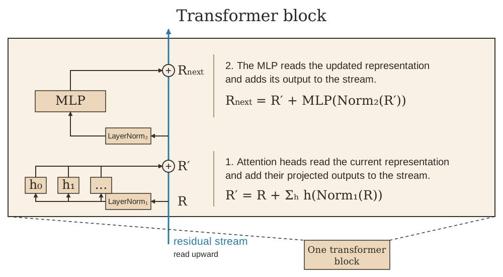
An update can change some readouts while leaving others unchanged. To isolate the geometry, consider a linear reader applied directly to one token’s stream vector . If a branch adds an update , then:
Such an update lies in the reader’s null space: the stream changes, but this reader cannot detect the change. Another reader may detect it. This connects residual updates to subspaces: features can occupy different directions or subspaces in the shared stream, and each reader is sensitive to particular directions. Those subspaces can overlap; residual addition does not guarantee separate, orthogonal compartments. The equation describes a direct linear readout; normalization before a transformer branch’s projection can change which updates are invisible to it.
This gives residual connections two related roles in a transformer. In backpropagation, the identity shortcut provides a direct gradient contribution around each attention or MLP branch. In the forward pass, it carries the current representation at each token position into the next addition.
In our “bank” example, the attention output is computed for the query position, “bank,” even when it reads information from “river.” Attention mixes information across positions rather than simply rearranging the tokens. The residual connection adds that update to the existing representation at “bank.” This follows the per-query attention computation and residual addition in Attention Is All You Need, §§3.1–3.2.
The shortcut therefore provides a direct route for a position’s own representation alongside information gathered from other positions. It carries the current representation, which may already include many updates, rather than restoring the original token embedding at every layer. This helps explain how context is added, but does not guarantee that token identity remains recoverable: updates can alter or cancel existing information. The MLP then computes another update separately at each position.
The original 2017 Transformer used post-norm: each sublayer computed . The equations above use pre-norm: normalization sits inside the branch, leaving the addition’s output on the direct path. These arrangements have different gradient behavior, as studied in On Layer Normalization in the Transformer Architecture. The simple sum over updates describes the pre-norm stream before any final normalization; it does not directly describe a stack that normalizes after every addition.
You can understand the addition without yet knowing how attention calculates its update. Our two-number example already showed the essential dependency: the second branch reads the result after the first branch’s contribution.
The stream has a fixed number of coordinates per position. It does not reserve a separate permanent slot for every layer’s result. Contributions can overlap, reinforce, or cancel, and addition alone does not ensure that earlier information remains recoverable. Inside a transformer block — mixing information and adding updates examines the components that compute those updates.
Depth as discrete time: the Euler connection
Each residual block moves a representation from its current point to a new point. That suggests viewing depth as a sequence of time steps:
Compare this with a differential equation that specifies a state’s rate of change:
Forward Euler approximates the next state by using the current rate for an interval of length :
The shared structure is current state plus an increment. We can interpret as the entire increment :
| Residual network | Euler interpretation |
|---|---|
| Representation | Current state |
| Block index | Discrete time index |
| Branch output | Increment over one step |
| Updated representation | Next state |
Setting gives the same algebraic form. Different branch parameters correspond to dynamics that can change with time. This interpretation connects neural-network depth to numerical integration; it appears explicitly in the Neural ODE paper’s introduction.
A finite residual network need not approximate a smooth continuous process accurately. Its updates can be large, its branches can differ abruptly, and CNN stage transitions can change the state dimension. The direct Euler analogy applies to fixed-dimensional additive steps; a final ReLU or normalization changes that update rule.
A stable differential equation can have an unstable Euler approximation
Take a scalar system:
Its exact solution is , which approaches zero. Euler gives:
Write . After steps, . The magnitude decays when , giving:
Here is the calculation for several choices, always starting from :
| Step size | Multiplier | First four states, starting at | Long-run behavior |
|---|---|---|---|
| Decays | |||
| Alternates and decays | |||
| Bounded oscillation; no decay | |||
| Alternates and grows |
Before changing the explorer, predict what happens as crosses . Use to compare , , and . Keep the equation and initial state fixed; record the multiplier and final magnitude.
Euler steps for dx/dt = −2x
Solid orange: Euler states · Dashed gray: exact solution e⁻²ᵗ at t = kh
Read all computed states
| Step k | Time kh | Euler xₖ | Exact e⁻²ᵏʰ |
|---|---|---|---|
| 0 | 0 | 1 | 1 |
| 1 | 0.75 | -0.5 | 0.2231 |
| 2 | 1.5 | 0.25 | 0.0498 |
| 3 | 2.25 | -0.125 | 0.0111 |
| 4 | 3 | 0.0625 | 0.0025 |
| 5 | 3.75 | -0.0313 | 5.53e-4 |
| 6 | 4.5 | 0.0156 | 1.23e-4 |
| 7 | 5.25 | -0.0078 | 2.75e-5 |
| 8 | 6 | 0.0039 | 6.14e-6 |
| 9 | 6.75 | -0.002 | 1.37e-6 |
| 10 | 7.5 | 9.77e-4 | 3.06e-7 |
| 11 | 8.25 | -4.88e-4 | 6.83e-8 |
| 12 | 9 | 2.44e-4 | 1.52e-8 |
| 13 | 9.75 | -1.22e-4 | 3.40e-9 |
| 14 | 10.5 | 6.10e-5 | 7.58e-10 |
| 15 | 11.25 | -3.05e-5 | 1.69e-10 |
| 16 | 12 | 1.53e-5 | 3.78e-11 |
The boundary is bounded but not asymptotically stable: it fails to reproduce the continuous solution’s decay. Above that boundary, the numerical states grow even though the underlying differential equation is stable. Stability and accuracy are also different: sends Euler’s state directly to zero after one step, while the exact solution at is .
Try a variation on paper: replace with , for a positive of your choice. Predict the interval of step sizes that makes the states decay, then check a value inside it and one outside. The multiplier becomes , so your interval should satisfy .
The same question becomes a Jacobian calculation
For the residual step , we already found:
A small perturbation evolves approximately as:
Across several blocks:
Backpropagation uses the transpose of this same product:
These equations explain the connection between sensitivity in the forward pass and gradients in the backward pass. A product that strongly amplifies some directions can amplify gradients; one that contracts them can suppress gradients. Our Jacobian article develops the local linear approximation behind this argument.
In the scalar Euler example, every block has derivative , so the product is simply . In a neural network, the Jacobians usually differ by depth and input. We must examine their products: eigenvalues of individual blocks alone do not generally determine how much a varying sequence of matrices can amplify a perturbation. Singular values describe the stretching of a particular product.
The identity term helps explain why a small branch derivative need not erase a gradient. It does not guarantee stability: if , the block’s Jacobian is zero; if , it is , doubling perturbations at every step. For blocks with a final activation or normalization, that operation’s Jacobian also belongs in the calculation.
This dynamical-systems approach was developed in work such as Haber and Ruthotto’s Stable Architectures for Deep Neural Networks. It connects numerical stability and gradient propagation, but does not make every residual network a simulation of a stable physical system. Nor is stability across depth the same question as whether parameter updates from an optimizer converge.
From discrete blocks to Neural ODEs
In 2018, Ricky T. Q. Chen, Yulia Rubanova, Jesse Bettencourt, and David Duvenaud introduced Neural Ordinary Differential Equations. Instead of specifying a fixed sequence of residual blocks, a Neural ODE parameterizes a continuous rate:
A numerical solver computes the final state from the initial state. Depending on the solver and its settings, it may evaluate the learned rate at adaptively chosen times. This is a model design built around continuous dynamics; an ordinary ResNet or transformer does not automatically use an ODE solver.
The connection gives us a useful way to inspect a deep model. Each branch writes a displacement into representation space, while its Jacobian describes how that update responds to nearby inputs. We can then ask which directions successive updates reinforce, which they cancel, and how those changes affect the model’s eventual output.