Build a tiny autograd engine in Python
A training loop needs the loss gradient to update a model’s parameters. Instead of deriving a new gradient formula for every model, we can teach a small engine the derivative rules for its basic operations and let it combine them through the computation graph.
We’ll build that engine in Python: a simplified version of the automatic differentiation machinery behind PyTorch’s torch.autograd. PyTorch operates on tensors, such as vectors and matrices. Our engine will operate on individual numbers so we can inspect every value and derivative.
The companion article develops the calculus behind this implementation. The three ideas we’ll use are:
- A partial derivative measures how the output responds to one input while the others stay fixed
- The chain rule connects derivatives along a path; contributions from different paths add
- Backpropagation applies those rules backward through a graph, starting with
We’ll build the engine in stages. First, our numbers will record a graph while running ordinary arithmetic. Then we’ll add gradient fields and fill them by hand. Finally, we’ll automate the same backward calculation. Each stage uses the same expression, so the graphs show exactly what changes. After checking the engine, we’ll use it to fit a line and train a small XOR network.
Run the arithmetic and record the graph
First, we need a class to store each number and record the inputs and operation that produced it. We’ll call it Value:
data: the numerical value_prev: the parent values used by the operation_op: the operation’s name, for drawing the graphlabel: a readable name such asaorL
There are no gradients yet. Addition and multiplication calculate their results immediately and attach the dependencies:
class Value:
    def __init__(self, value, label=''):
        self.data = float(value)
        self._prev = ()
        self._op = None
        self.label = label

    def __add__(self, other):
        out = Value(self.data + other.data)
        out._prev = (self, other)
        out._op = '+'
        return out

    def __mul__(self, other):
        out = Value(self.data * other.data)
        out._prev = (self, other)
        out._op = '*'
        return out
Both operands must be Value objects at this stage. Try a single addition:
a = Value(2, label='a')
b = Value(3, label='b')

total = a + b
total.label = 'sum'

print(total.data)  # 5.0
We can visualize the recorded computation as a graph, with a and b feeding into the addition that produces sum:

Let’s now connect several operations. For that, we’ll use:
with , , , and . Here names the function’s final output, which we want to differentiate with respect to its inputs.
a = Value(2, label='a')
b = Value(-3, label='b')
c = Value(10, label='c')
f = Value(-2, label='f')

d = a * b
d.label = 'd'
e = c + d
e.label = 'e'
L = e * f
L.label = 'L'

print(L.data)  # -8.0
When we visualize this computation, we can follow the intermediate values and through to the final output :
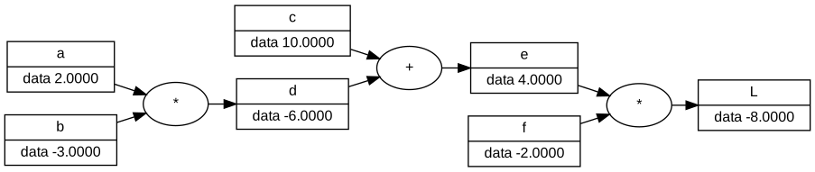
We store _prev as a tuple so operand order and repeated operands are retained. In a * a, both entries refer to the same object. A set can record which nodes are connected, but it would collapse those two operand occurrences. That distinction will matter when we accumulate derivatives.
Draw these graphs with Graphviz
The diagrams above were generated from these Python objects. Install the Graphviz application, which provides the dot command, and its Python wrapper:
python -m pip install graphviz
dot -V
The Python package alone does not install dot. Save the drawing helper as graphviz_view.py beside your example. It walks backward through the dependencies, draws each value as a record, and inserts a separate node for each operation:
from graphviz import Digraph, escape


def trace(root):
    nodes, edges, seen = [], [], set()

    def build(node):
        if node in seen:
            return
        seen.add(node)
        nodes.append(node)
        # Early stages store parents; the final engine stores weighted edges.
        parents = (parent for parent, _ in node.edges) if hasattr(node, 'edges') else node._prev
        for parent in parents:
            edges.append((parent, node))
            build(parent)

    build(root)
    return nodes, edges


def draw_dot(root):
    dot = Digraph(format='svg', graph_attr={'rankdir': 'LR', 'ranksep': '0.3'})
    dot.attr('node', fontname='Arial', fontsize='12')
    nodes, edges = trace(root)
    ids = {node: f'n{i}' for i, node in enumerate(nodes)}
    for node in nodes:
        uid = ids[node]
        label = escape(node.label).replace('{', r'\{').replace('}', r'\}').replace('|', r'\|').replace('<', r'\<').replace('>', r'\>')
        fields = [label, f'data {node.data:.4f}']
        if hasattr(node, 'grad'):
            fields.append(f'grad {node.grad:.4f}')
        dot.node(uid, label=' | '.join(fields), shape='record')
        if node._op:
            dot.node(uid + '_op', label=node._op, shape='ellipse')
            dot.edge(uid + '_op', uid)
    for parent, node in edges:
        target = ids[node] + ('_op' if node._op else '')
        dot.edge(ids[parent], target)
    return dot
Then draw any result:
from graphviz_view import draw_dot

draw_dot(L).render('forward-graph', cleanup=True)  # writes forward-graph.svg
# In a Jupyter notebook, display the returned object directly:
# draw_dot(L)
The helper includes a gradient field only when the object has one. It also supports the final engine’s edges representation, so we can use it at every stage. Graphviz is only for visualization; the arithmetic and autograd engine run without it.
Add gradients and propagate them by hand
Keep the arithmetic methods unchanged and add grad to the constructor:
    def __init__(self, value, label=''):
        self.data = float(value)
        self._prev = ()
        self._op = None
        self.label = label
        self.grad = 0.0
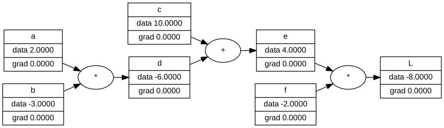
Rebuild the example with this updated class. Each grad field starts at zero as an accumulator; we have not yet calculated the derivatives. The field will hold the derivative of the final output with respect to that node, including intermediate nodes such as and .
In this scalar engine, each .grad field stores one partial derivative, such as . We use “gradient” as shorthand for that stored derivative; the full parameter-gradient vector collects the derivatives with respect to all trainable parameters.
Seed L.grad with , because . Then follow the graph backward, multiplying the derivative of with respect to each result by that result’s local derivative with respect to an input:
L.grad = 1.0

# L = e * f
f.grad += e.data * L.grad  # 4
e.grad += f.data * L.grad  # -2

# e = c + d
c.grad += 1.0 * e.grad     # -2
d.grad += 1.0 * e.grad     # -2

# d = a * b
a.grad += b.data * d.grad # 6
b.grad += a.data * d.grad # -4
The multiplication of .data and .grad here is an application of the chain rule. For example, a.grad += b.data * d.grad follows the path from through to :
d.grad tells us how sensitive the final output is to . The local derivative tells us how sensitive is to ; because , that derivative equals the other operand’s value, b.data. Multiplying the two connects ‘s effect on to ‘s effect on .
The general rule is the derivative of the final output with respect to this node × the local derivative of this node with respect to its input. Both factors are derivatives; they describe different parts of the path. The local derivative happens to be the other operand’s .data for multiplication. For addition, it is , which explains c.grad += 1.0 * e.grad. At the final multiplication, e.grad += f.data * L.grad uses the same rule, starting from .
We use += so contributions can accumulate when a value feeds more than one operation. The diamond example below will show why overwriting a contribution or propagating it too early gives the wrong result. Run these updates once on the fresh graph. Select , then use to inspect the graph after each backward step:
| Value | Forward data | Derivative of |
|---|---|---|
The intermediate gradient magnitudes are needed to calculate the gradients farther backward. For example, d.grad = -2 combines with the multiplication’s local derivative :
Keeping only the sign of d.grad would replace with and give , losing the correct sensitivity. Backpropagation needs the actual derivative values; the optimizer later decides how to use the resulting parameter gradients. Intermediate values such as and are recomputed from the parameters, rather than updated as independent parameters themselves.
Our teaching engine keeps every grad field visible so we can inspect the calculation. Retaining intermediate gradients for inspection is a separate implementation choice; PyTorch provides retain_grad() to request it.
Backward propagation fills in the gradients; it does not change any data values. For example, a.grad = 6 says a small increase in should increase by about six times that amount. We can check this by actually perturbing while keeping the other inputs fixed:
def numeric_loss(a, b=-3, c=10, f=-2):
    return (a * b + c) * f

h = 0.1
before = numeric_loss(a.data)      # -8.0
after = numeric_loss(a.data + h) # approximately -7.4
estimate = (after - before) / h # approximately 6.0
assert abs(a.grad - estimate) < 1e-10
The after calculation uses ; using the unchanged input twice would give zero. Here the estimate agrees up to floating-point rounding because is linear in when , , and are fixed. This extra evaluation checks our hand-calculated gradient. The backward steps themselves used only values already stored in the graph.
Save local derivatives on the edges
The manual calculation worked because we supplied each operation’s derivative rule and chose the backward order ourselves. To automate it, each operation will record (parent, local_derivative) pairs in edges instead of only parent references in _prev.
For addition, both local derivatives are . For multiplication, each is the other operand’s current value. grad still holds the derivative of the final output, while the number stored on an edge is only a local derivative.
Replace the earlier class with this version:
class Value:
    def __init__(self, data, edges=(), label='', op=None):
        self.data = float(data)
        self.grad = 0.0
        self.edges = tuple(edges)  # (parent, local derivative) pairs
        self.label = label
        self._op = op

    @staticmethod
    def wrap(value):
        return value if isinstance(value, Value) else Value(value)

    def __add__(self, other):
        other = Value.wrap(other)
        return Value(self.data + other.data, ((self, 1.0), (other, 1.0)), op='+')

    def __mul__(self, other):
        other = Value.wrap(other)
        return Value(self.data * other.data,
                     ((self, other.data), (other, self.data)), op='*')
wrap lets arithmetic accept ordinary numbers as well as Value objects. Labels and operation names remain available for Graphviz. Nothing propagates backward yet: the forward pass now records both the dependencies and the numerical factors that a backward pass will need.
Visit the graph in the right order
The output already knows which values it depends on, so why not propagate its gradient and immediately recurse into each input? That works for our first graph, where each intermediate value is used only once. A shared intermediate value needs more care: its gradient must collect all downstream contributions before we propagate it farther backward.
Why a shared value needs both accumulation and ordering
Consider a diamond-shaped dependency graph. We make a an intermediate result rather than a leaf, so we can see what happens when its incomplete gradient reaches an earlier input:
x = Value(1, label='x')
a = x * 2
a.label = 'a'
b = a * 3
b.label = 'b'
c = a + 1
c.label = 'c'
d = b + c
d.label = 'd'
Here a feeds two later operations: b and c. In our code, parents means a node’s input dependencies: a is a parent of both b and c. We call b and c its consumers. The ordering problem comes from multiple consumers sharing a value, not simply from an operation having two inputs.
The arrows below show forward dependencies, and their labels give local derivatives. The gradient fields show the completed backward pass, with d.grad = 1. Constant inputs are omitted to make the diamond visible:
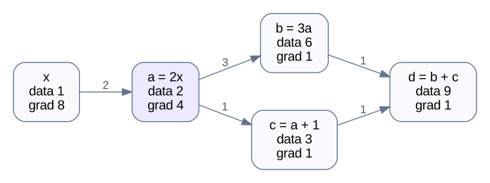
Working backward, d = b + c contributes 1 to both b.grad and c.grad. The two branches then contribute to a.grad:
a.grad += 3 * b.grad  # contribution from b: 3
a.grad += 1 * c.grad  # contribution from c: 1
# a.grad is now 4
x.grad += 2 * a.grad  # 8
+= preserves both contributions. Using = for each branch would leave a.grad equal to whichever contribution arrived last: 1 or 3, instead of 4.
Ordering ensures we propagate the complete sum. Suppose an immediate recursive walk processes d, then b, then a, before reaching c. When it processes a, only the contribution from b has arrived, so it sends 2 × 3 = 6 to x.grad. If a visited set prevents processing a again, the contribution through c never reaches x. Simply revisiting a is also wrong if we propagate its accumulated gradient again: after c arrives, that would add 2 × 4 = 8 to the existing 6, giving 14 instead of 8.
Build the order before propagating gradients
A topological order places every input dependency before the operations that use it. Ignoring constant nodes, both [x, a, b, c, d] and [x, a, c, b, d] are valid. There is no dependency between b and c, so either can come first. Reversing either order processes d first, both branches before a, and a before x.
To construct that order, a depth-first traversal visits a node’s parents before appending the node itself. A seen set adds each node only once. This traversal only builds the list; it does not propagate gradients yet. The later backward loop processes the reversed list, so a shared node runs once, after all its consumers have contributed.
The order of the two branches can depend on how we iterate over the stored inputs. Either order adds 3 and 1 to a.grad, giving 4. In general, floating-point addition can introduce small rounding differences, but neither ordering loses a path. Shared values are common in neural networks: for example, one activation can feed several neurons in the next layer.
Add this method to Value:
    def backward(self):
        order, seen = [], set()

        def visit(node):
            if node in seen:
                return
            seen.add(node)
            for parent, _ in node.edges:
                visit(parent)
            order.append(node)

        visit(self)
        for node in order:
            node.grad = 0.0
        self.grad = 1.0
        for node in reversed(order):
            for parent, local_derivative in node.edges:
                parent.grad += node.grad * local_derivative
There are three separate steps: clear old gradients in the reachable graph, seed the final output’s gradient with one, and traverse backward to accumulate contributions. The inner loop replaces each hand-written update with the same general rule: parent.grad += node.grad * local_derivative.
Rebuild the same graph using this class, then call:
L.backward()
print(a.grad, b.grad, c.grad, f.grad)  # 6.0, -4.0, -2.0, 4.0
draw_dot(L).render('automatic-backward', cleanup=True)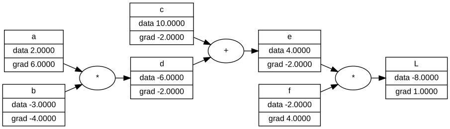
The diamond uses the same backward pass. After rebuilding its values with this updated class:
d.backward()
print(d.data)          # 9.0
print(b.grad, c.grad)  # 1.0, 1.0
print(a.grad, x.grad)  # 4.0, 8.0
The seen set deduplicates nodes, while edges preserves every operand occurrence. In a * a, two edges point to the same parent. Both execute their += update. Replacing edges with a set of parents without retaining the corresponding contributions would lose that distinction.
Our backward() deliberately clears reachable gradients on each call. This makes repeated calls on the same unchanged graph reproducible. It differs from APIs that accumulate leaf gradients across backward calls and require a separate zeroing step. Within one backward pass, contributions still accumulate from all graph paths.
This implementation saves numeric local derivatives during the forward pass. Change parameter data after backward, then build a fresh graph for the next iteration. Rerunning backward on an old graph after changing data would use stale local derivatives.
The recursive graph traversal keeps this teaching engine short. Long computation chains, such as a loss summed over thousands of examples, can exceed Python’s recursion limit; an iterative traversal avoids that limit.
Add the operations our models will use
The graph and backward traversal already work. To support the models below, put import math at the top of the file, then add positive integer powers and the hyperbolic tangent, tanh, to Value:
    def __pow__(self, exponent):
        if not isinstance(exponent, int) or exponent < 1:
            raise ValueError("This engine supports positive integer powers only")
        return Value(self.data ** exponent,
                     ((self, exponent * self.data ** (exponent - 1)),), op=f'**{exponent}')

    def tanh(self):
        output = math.tanh(self.data)
        return Value(output, ((self, 1.0 - output * output),), op='tanh')
Powers let (prediction - target) ** 2 record a square operation. Restricting them to positive integers covers our examples without introducing domains such as fractional powers of negative numbers. The smooth activation tanh has derivative and lets the network express nonlinear relationships.
Python’s convenience operators support negation, subtraction, expressions such as 2 * w, and sum(...):
    def __neg__(self):
        return self * -1.0

    def __sub__(self, other):
        return self + -Value.wrap(other)

    def __rsub__(self, other):
        return Value.wrap(other) + -self

    __radd__ = __add__
    __rmul__ = __mul__
These methods all belong inside Value. You can download the stages separately: forward_graph.py, manual_gradients.py, and the complete tinygrad.py. Keep the first two in the same directory because the manual version reuses the example-building function. To regenerate every diagram, save graphviz_view.py and render_graphs.py there too, then run python render_graphs.py with Graphviz installed.
Check the engine against the arithmetic
For the model , take , , , and . The squared loss is . The chain rule gives and . We can now check that the engine reproduces those values.
Save the complete file as tinygrad.py. In another Python file in the same directory:
from tinygrad import Value

w, b = Value(1), Value(0)
prediction = w * 2 + b
loss = (prediction - 5) ** 2
loss.backward()

print(loss.data)  # 9.0
print(w.grad)     # -12.0
print(b.grad)     # -6.0

a = Value(3)
q = a * a + a
q.backward()
print(a.grad)    # 7.0: all three paths contribute
The engine never received a special formula for this model’s weight gradient. It recorded multiplication, addition, subtraction, and a square, then combined their local derivatives.
Use finite differences to check the result
Finite differences provide an independent check of our backward pass. If you need a refresher, the companion article explains how nearby function values estimate a derivative. The engine has already obtained w.grad from the recorded operations at . To check its implementation, evaluate the loss separately on both sides of that weight:
def numeric_loss(weight):
    return (weight * 2 - 5) ** 2

h = 1e-5
finite_difference = (numeric_loss(1 + h) - numeric_loss(1 - h)) / (2 * h)
assert abs(w.grad - finite_difference) < 1e-6
This central difference is a numerical check, not the engine’s differentiation algorithm. Checking every parameter this way needs two evaluations per parameter. Reverse-mode automatic differentiation instead reuses a single recorded graph to compute all parameter gradients for a scalar output, with work proportional to the graph’s size.
We choose a central difference because sampling both sides cancels the leading approximation error. For sufficiently smooth functions, forward and backward differences typically have error proportional to , while central difference has error proportional to . Halving therefore roughly halves the one-sided error but reduces central-difference error to about a quarter. For our quadratic loss, central difference is exact in exact arithmetic; for general functions, it remains an approximation.
Extremely small values of eventually introduce floating-point cancellation, so smaller is not always better for this numerical check. The training loops below obtain their gradients by calling backward() on the current graph. With the engine checked, we can examine how the choice of loss affects those gradients and then use them to update parameters.
The choice of loss changes the learning signal
The model tells us how its prediction responds to a weight. The loss tells us how much that prediction change matters to the objective.
For the same prediction, compare two losses:
| Loss | Derivative with respect to prediction | Derivative with respect to weight |
|---|---|---|
| Squared error: | ||
| Absolute error: | , away from zero | , away from zero |
At our starting point, the prediction gradient is for squared error and for absolute error. Multiplying by the same model derivative, , gives weight gradients and .
Switch between and below. Move while watching both the prediction gradient and the weight gradient. The input stays fixed, so only the first factor changes.
x = 2, y = 5, and b = 0 stay fixed. This experiment updates only w.
Squared error produces a larger prediction gradient when the error’s magnitude is larger. Absolute error has constant gradient magnitude with respect to the prediction whenever the error is nonzero. Its derivative is undefined at zero; the widget selects a subgradient of zero there.
Neither loss supplies the rules for differentiation. Those rules come from calculus. The choice of loss determines the function those rules act on, and therefore the initial signal propagated through the model.
A derivative becomes an update
Gradient descent subtracts a scaled gradient:
The learning rate scales the gradient, so both determine the update size. Plain stochastic gradient descent (SGD) uses the same update rule with a gradient calculated from a sampled example or minibatch. With squared error, , and :
Holding the bias at zero, the new prediction is and the new loss is . Use and in the loss experiment to reproduce this calculation.
Here we updated only the weight. If we also update the bias from the same gradient, it becomes , giving prediction and loss zero for this single example. These are different updates, so they produce different results.
A negative derivative suggests increasing the parameter; a positive derivative suggests decreasing it. That is a local statement. A large step can pass a minimum and increase the loss. Backpropagation calculates the gradient; the optimizer and its learning rate determine what to do with it.
Other optimizers transform the gradients before updating parameters. For example, Adam uses moving averages of gradients and squared gradients to rescale the updates for individual parameters. Its update need not point along the current negative gradient. This changes the optimization rule; backpropagation still supplies the derivative values.
Why we recalculate gradients after an update
The update moves the weight, but the gradient was evaluated at its previous value. The chain rule combines derivative rules, and the numbers those rules produce can change after that move. Let’s reuse our loss and let its input come from a multiplication: . Keep fixed and treat as the weight we adjust:
The multiplication gives , and the loss gives . Combining them:
At , we get and , so the gradient is . If an update moves to , then becomes and the gradient becomes :
| Weight | Intermediate value | Loss derivative | Weight gradient |
|---|---|---|---|
The rules stay the same, but their numerical values can change after an update. The multiplication’s derivative stays because is fixed; the loss derivative changes with . Reusing the old gradient of at would describe the slope at the previous weight, not the current one.
Move below to see these values change. From the initial weight of , select to move to and recalculate the gradient. This demonstration uses learning rate , so each update subtracts one sixteenth of the current gradient from the weight.
Learning rate η = 1/16: w ← w − η × (dL/dw). The intermediate value, loss, and gradient are recalculated after each update.
This connects the two senses in which we refer to derivatives and approximations as local. Each operation supplies a local derivative rule. The resulting gradient describes the loss near the current weight and gives a local approximation of its change. After updating the weights, our engine builds a fresh graph and computes a new gradient. We can now repeat that process to train on several examples.
Learn from several examples
Let’s revisit the line-fitting task from our earlier article, this time using our engine to calculate the gradients. One training example cannot determine a unique line: many pairs satisfy . Add more examples:
| Input | Target |
|---|---|
| 0 | 1 |
| 1 | 3 |
| 2 | 5 |
| 3 | 7 |
These points lie on , so we can check whether training finds and .
Define the loss as the mean of the four squared errors:
The shared weight appears in all four predictions. During backward, each path contributes to the same w.grad. Multiplication by scales all contributions to match the mean loss. Summing instead of averaging would multiply both gradients by four.
Use to inspect one update, then . Try learning rate from the reset state to see loss grow even though the gradients are calculated correctly.
Each click builds a fresh graph, averages four squared errors, runs backward(), and updates both w and b. The line plot rescales if the parameters grow; the loss plot uses log₁₀, with a floor of 10⁻¹².
The widget uses a JavaScript counterpart of the scalar engine above. Its gradients are calculated through a new graph on each step. Here is the same training loop in Python:
def train_line(steps=1000, learning_rate=0.05):
    data = [(0, 1), (1, 3), (2, 5), (3, 7)]
    w, b = Value(-1), Value(0)
    for _ in range(steps):
        loss = sum((w * x + b - y) ** 2 for x, y in data) * (1 / len(data))
        loss.backward()  # also clears this graph's old gradients
        for parameter in (w, b):
            parameter.data -= learning_rate * parameter.grad
    final_loss = sum((w.data * x + b.data - y) ** 2 for x, y in data) / len(data)
    return w.data, b.data, final_loss
Both gradients come from the same forward pass before either parameter changes. The next iteration recomputes predictions, loss, and derivatives at the updated parameters. The returned loss is evaluated after the last update, so it describes the returned weights.
Use the same engine for a neural network
So far, the model has been affine. We’ll now train a small network on XOR to demonstrate that the same engine handles a nonlinear model with a hidden layer. Its forward pass is a larger composition of the operations we already support, so it needs no new differentiation machinery.
One neuron: weighted sum, then activation
A neuron first combines its inputs into one number, then applies an activation function:
Here, is one input, is its learned weight, is the learned bias, and is the activation function. The output is a single scalar; we keep for the target. In this section, indexes the inputs to one neuron, rather than the training examples in the previous section.
The dot product multiplies corresponding entries and sums them. Adding the bias makes an affine transformation from to . Applying a nonlinear activation such as ReLU, sigmoid, or tanh lets layers compose nonlinear functions. Our earlier model is the one-input case with the identity activation .
For a concrete example, take three inputs:
First compute the weighted sum plus bias:
With ReLU, the output would be . Our engine uses tanh, so its nonlinear neuron instead returns:
The inputs, weights, and bias determine ; the activation determines how that value is passed forward.
Follow the chain rule through the neuron
Attach a loss to this neuron’s output. A weight affects that loss through the weighted sum and the activation:
The local derivative of the weighted sum with respect to is . The activation contributes . Multiplying these by the loss sensitivity arriving at the output gives:
For the bias, , so:
For tanh, . If this single neuron predicts a target and we use squared error, , then:
Return to the three-input example and choose target . At , the activation slope is approximately . For the first weight:
A small increase in therefore reduces the loss locally. Compared with our earlier affine model, the chain has one additional factor: the activation’s slope. With the identity activation, that factor is , recovering the earlier formula.
For a hidden neuron, arrives from the later layers. To continue backward, this neuron contributes to the gradient of input . If an input feeds several neurons, their contributions add, just as they did in our earlier graph examples.
From one neuron to a layer
A layer with neurons has one weight vector and one bias per neuron. Stack the weight vectors as the rows of and the biases into :
Here, collects the layer’s outputs, and acts on each entry separately. An MLP feeds those outputs into the next layer.
The code below implements the same two stages: total is , and total.tanh() applies the activation. We keep the final layer linear for this regression example:
import random


class Neuron:
    def __init__(self, n_inputs, rng, nonlinear=True):
        self.weights = [Value(rng.uniform(-1, 1)) for _ in range(n_inputs)]
        self.bias = Value(0)
        self.nonlinear = nonlinear

    def __call__(self, inputs):
        total = sum((w * x for w, x in zip(self.weights, inputs)), self.bias)
        return total.tanh() if self.nonlinear else total

    def parameters(self):
        return self.weights + [self.bias]


class MLP:
    def __init__(self, sizes, seed=42):
        rng = random.Random(seed)
        self.layers = [
            [Neuron(n_in, rng, nonlinear=i < len(sizes) - 2)
             for _ in range(n_out)]
            for i, (n_in, n_out) in enumerate(zip(sizes, sizes[1:]))
        ]

    def __call__(self, inputs):
        for layer in self.layers:
            inputs = [neuron(inputs) for neuron in layer]
        return inputs

    def parameters(self):
        return [p for layer in self.layers for neuron in layer
                for p in neuron.parameters()]
MLP([2, 4, 1]) creates two inputs, four hidden neurons with tanh, and one linear output. Its parameters are 8 hidden weights, 4 hidden biases, 4 output weights, and 1 output bias: 17 trainable scalars.
Train it on XOR, encoding equal inputs as and different inputs as . No affine function of two inputs can fit all four targets exactly; the hidden nonlinear activations allow the model to fit them.
def train_xor(steps=1000, learning_rate=0.1):
    # Same inputs twice equal -1; different inputs equal +1.
    examples = [([0, 0], -1), ([0, 1], 1), ([1, 0], 1), ([1, 1], -1)]
    model = MLP([2, 4, 1], seed=42)
    parameters = model.parameters()
    for _ in range(steps):
        loss = sum((model(x)[0] - y) ** 2 for x, y in examples) * 0.25
        loss.backward()
        for parameter in parameters:
            parameter.data -= learning_rate * parameter.grad
    predictions = [model(x)[0].data for x, _ in examples]
    final_loss = sum((p - y) ** 2 for p, (_, y) in zip(predictions, examples)) / 4
    return predictions, final_loss
The training structure is unchanged: build predictions and a scalar loss, call backward(), and update parameters. The engine sees operations and edges. It does not need to know which operations belong to a neuron or a layer.
Run the complete file:
python3 tinygrad.pyWith the supplied seed, 1,000 steps, and learning rate , the XOR predictions round to [-1.0, 1.0, 1.0, -1.0] at four decimal places. This is a small demonstration with fixed data and initialization, rather than a guarantee for arbitrary networks or learning rates.
When gradients vanish, explode, or become zero
The chain rule also explains why a neuron may learn slowly or stop receiving a learning signal. Each path multiplies local derivatives together, so a zero factor blocks that path, while repeated small or large factors can shrink or amplify its contribution.
Consider a neuron with a ReLU activation:
For positive , the activation’s derivative is . For negative , it is . At , ReLU is not differentiable; implementations commonly choose a derivative value of zero. When is negative, the weight gradient becomes:
The bias gradient is zero too. This example therefore supplies no gradient update to the neuron’s incoming weights or bias through this activation. If the ReLU stays inactive for every training example, it can become a dying ReLU: it consistently outputs zero and blocks the gradient needed to change its incoming parameters. With fixed inputs and ordinary gradient descent, it cannot recover through these gradients alone. In a hidden layer, changes in earlier layers can still change its inputs. Stanford’s CS231n notes discuss this failure mode and how Leaky ReLU retains a small nonzero slope for negative inputs.
A zero derivative for one example does not mean the neuron is dead—it may activate for another. Nor does a zero loss gradient necessarily indicate a dead neuron: it can occur at a stationary point, including a minimum.
Gradients can also become very small or very large without any factor being zero. Along a simplified path with ten local derivative factors, starting with an incoming gradient of :
| Local factors along the path | Product | Effect |
|---|---|---|
| Ten factors of | The gradient contribution shrinks | |
| Ten factors of | The gradient contribution grows |
Repeated shrinking can produce vanishing gradients, leaving earlier parameters with very small updates. Repeated amplification can produce exploding gradients, making updates unstable or causing numerical overflow. In a network, these factors include weights as well as activation derivatives, and contributions from different paths add together. The table illustrates one path rather than predicting the whole network’s gradient. The Deep Learning textbook explains these training difficulties in more detail.
Our engine uses tanh, whose derivative is . When its output is close to or , this derivative is close to zero, so it can shrink gradients even without ReLU’s flat negative region. This is activation saturation, distinct from a dying ReLU. Autodiff calculates these derivatives correctly; it does not guarantee that they will be large enough for useful learning or small enough for stable updates.
From an arithmetic graph to a trainable model
We started with values that could record arithmetic, added derivative fields, and filled them by hand. Recording local derivatives and visiting nodes in reverse order automated the same calculation.
The engine needed derivative rules for its basic operations, not a separate derivative formula for each model. A forward pass recorded values and local derivatives; a backward pass combined their contributions, including every path through a reused value. The loss supplied the objective, and gradient descent used its parameter gradients to update the model. Each new update required a fresh computation at the new parameters.
We verified that calculation against both hand-derived answers and finite differences, then used the same engine to train a line and a small neural network. Increasing the model’s complexity changed the computation graph; the differentiation machinery stayed the same.
For the broader neural-network treatment, see How neural networks learn: backpropagation and gradient descent. For a complementary implementation that attaches backward functions to operations, see Karpathy’s micrograd engine and his Neural Networks: Zero to Hero materials.