Floats, bfloat, and how bits shape model memory
Underneath all the abstraction, a neural network is a large collection of numbers called parameters — the weights and biases each neuron carries across every layer, which we walked through in detail in the article on how networks learn. The parameter count tells you how many of those numbers the model stores; the numeric format tells you the size of each one in bytes. Multiply them and you get the model’s memory footprint — the first number you need before you pick hardware, pick a precision, or decide whether the thing fits on one GPU at all.
Take the small network we trained in the MNIST article — a dense classifier with two Keras Dense layers: 784 flattened pixel inputs feed into a 128-neuron hidden layer, which feeds into a 10-neuron output layer (one per digit).
The shorthand for this shape is 784 → 128 → 10, where 784 is the input size, not a layer. The parameter count adds up to:
Keras stores each parameter as fp32 — 32-bit floating point, 4 bytes each — by default. So the trained model occupies in memory when loaded. But this is a toy model built for learning — small enough that you could email it. Real-world models are orders of magnitude larger, and that’s where the number of parameters starts to matter.
Every model published on a hub like Hugging Face ships with a model card — the public README sitting next to the weights file, summarising what the model is, how it was trained, and the two numbers we care about here: how many parameters it has and what numeric format each one is stored in.
Let’s take a state-of-the-art open-source OCR model — open PaddleOCR-VL on Hugging Face and the sidebar tells you both things we care about: the number of parameters and the format each one is stored in.
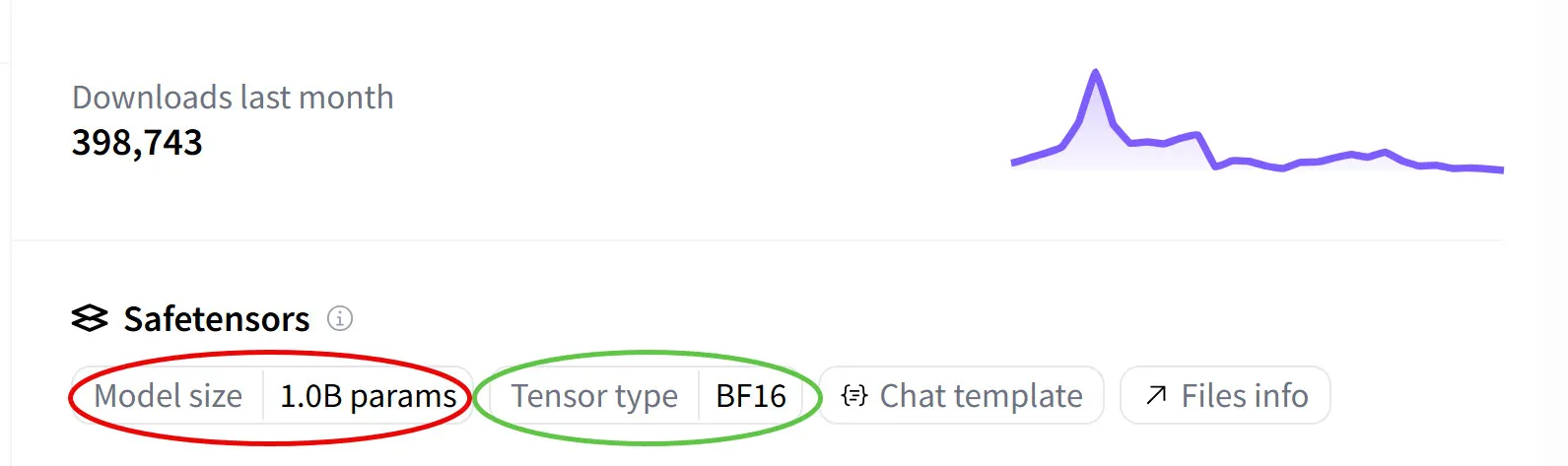
Model size is the total parameter count — how many numbers the model stores. Tensor type is the dtype — short for data type.
The d is there to distinguish it from plain type: in Python, type(x) tells you about the container (list, numpy.ndarray, torch.Tensor), whereas dtype tells you about the elements inside it (float32, int8, bfloat16) — and that’s the thing that decides how many bytes each weight occupies.
The term started in NumPy and every ML framework picked it up.
In code, you read it off any tensor or array through its .dtype attribute — and every framework reports it the same way, as the canonical name of the format:
>>> import torch
>>> torch.tensor([0.5], dtype=torch.bfloat16).dtype
torch.bfloat16

>>> import numpy as np
>>> np.array([0.5], dtype=np.float16).dtype
dtype('float16')
Hugging Face reads the same information straight from the safetensors file — safetensors is Hugging Face’s file format for saving and distributing trained model weights, and the dtype of each tensor is stored in its metadata, which is what the sidebar displays as “Tensor type”.
BF16 in the sidebar means every weight in the model is a bfloat16 — “Brain Float 16” — a 16-bit floating-point format designed at Google for ML. It’s a float-like format — same sign/exponent/mantissa structure as an IEEE-754 float, just packed into 16 bits instead of 64, with its own split between exponent and mantissa.
We’ll look closely at the differences — including why bf16 isn’t the same thing as IEEE-754 float16 despite both being 16 bits — later in the article.
So the steps to compute the model’s memory footprint are the same ones we used for MNIST, just with bigger numbers. The 1.0B figure is the sum of parameters across every layer of the model — the same per-layer arithmetic we did by hand for MNIST, except Hugging Face has already done it for us by walking every tensor in the safetensors file and adding up the element counts.
So the card says 1 billion params (“B” is shorthand for billion, ). Multiply that by 2 bytes per bf16 weight and we get the model’s weight footprint:
This is the dominant memory cost at inference, where activations are transient (only one layer’s worth lives in memory at a time during the forward pass) and the KV cache, when present, is usually smaller than the weights for typical workloads. Training is a different story — the same model needs the weights plus gradients, optimizer state, and cached activations for backprop — which we’ll quantify in a dedicated section below.
Now scale the same arithmetic up and the stakes change fast. A 7B-parameter model takes 28 GB at fp32 — doesn’t fit on a 24 GB RTX 4090 at all, and leaves barely 4 GB of headroom on a 32 GB RTX 5090 (not enough for activations and the KV cache). At 14 GB in fp16 it fits comfortably on either; 7 GB in int8 leaves room to spare. A 70B model at fp16 is 140 GB — no single GPU holds it, and the format choice starts dictating whether you need one GPU, two, or eight.
Although the default format in training frameworks is fp32, models are often published in something narrower: teams routinely trade some of the precision they trained with for smaller downloads and lower VRAM cost at inference. The trade takes two broad forms — dropping to a 16-bit floating-point format (fp16, bf16) or going further with quantization, mapping weights to a small set of discrete levels, usually at 8 or 4 bits. Had the authors published PaddleOCR-VL in fp32, the same model would occupy 4 GB. They picked bf16 because it halves the memory vs fp32 with effectively no quality loss — we’ll walk through why that choice works in the rest of the article.
Not every number in a network is a weight
Model weights aren’t the only numbers in a running network. A full picture has several distinct categories — each consuming memory, each free to pick its own format. You can learn more about where each one originates — weights and biases, layer activations during the forward pass, gradients during the backward pass, and the optimizer’s update step — in the article on how networks learn.
Two of them are universal: weights and activations exist whether you’re running inference or training. The weights are the trained parameters themselves — fp32 historically, bf16 or fp16 today, or quantized down to 8 or 4 bits for inference at scale. The activations are intermediate outputs from each layer during the forward pass — transient at inference (only one layer’s output is alive in memory at a time, since each layer’s input is just the previous layer’s output), cached for the backward pass at training (every layer’s outputs have to stay alive so backprop can reuse them), and usually stored in the same format as the weights.
At inference, transformer-based LLMs also carry a KV cache — keys and values cached across past tokens during autoregressive generation, so attention doesn’t have to recompute them for every new token. Often kept in fp16 or fp8 to save memory across long contexts.
During training, two more categories enter the picture:
- Gradients — derivatives computed during the backward pass to update weights. Span many orders of magnitude (small magnitudes especially), which is why range matters here and why bf16 (and later fp8 E5M2) win for them.
- Optimizer state — Adam keeps two moments per parameter, so 2× the parameter count. Almost always fp32 even when weights live in bf16, because small drift accumulates across thousands of training steps.
In code, dtype lives in a few specific places. Here’s the relevant excerpt from our training MNIST article:
# Input data — explicitly cast to float32
X_train = train_images.reshape(-1, 784).astype("float32") / 255.0

# Model — Dense layers default to fp32 for weights and biases (no dtype= passed)
model = keras.Sequential([
    keras.layers.Dense(128, activation="relu", input_shape=(784,)),
    keras.layers.Dense(10, activation="softmax"),
])

# Optimizer — owns its own state, allocated separately
model.compile(
    optimizer=keras.optimizers.SGD(learning_rate=0.1),
    loss="sparse_categorical_crossentropy",
    metrics=["accuracy"],
)
Three different lines, three different categories. .astype("float32") sets the input data dtype, which then propagates into activations as values flow forward through the layers. The Dense(...) constructors do not require a dtype= argument — Keras defaults to fp32 for weights and biases. To override that default, you’d pass dtype= explicitly:
# Same architecture, but weights and biases stored in bf16
model = keras.Sequential([
    keras.layers.Dense(128, activation="relu", input_shape=(784,), dtype="bfloat16"),
    keras.layers.Dense(10, activation="softmax", dtype="bfloat16"),
])
# PyTorch equivalent — nn.Linear takes the dtype directly
model = nn.Sequential(
nn.Linear(784, 128, dtype=torch.bfloat16),
nn.ReLU(),
nn.Linear(128, 10, dtype=torch.bfloat16),
)Both forms only override the weights and biases dtype — they do nothing to activations, gradients, or optimizer state. The optimizer is constructed independently and owns the dtype for its optimizer state: plain SGD has none, but Adam would allocate two fp32 moments per parameter. Mixed-precision wrappers like torch.amp.autocast and GradScaler decouple these categories further — for example running the forward pass in bf16 while keeping parameters in fp32. So picking a layer’s dtype= answers exactly one question: what format the weights are stored in. The rest is decided independently.
This is what people mean by mixed-precision training and inference: a single model deliberately uses different formats for different roles, each picked for its numerical demands. For the rest of the article, when we say “the model is in bf16”, we usually mean the weights are in bf16. The other roles may sit above or below that.
To estimate the actual memory bill at training, you stack up the per-parameter cost. The standard mixed-precision recipe — bf16 weights with an fp32 gradient-descent optimizer (Adam being the most common) — works out to 16 bytes per parameter before activations:
- bf16 weights: 2 bytes
- bf16 gradients: 2 bytes (same shape as weights)
- fp32 Adam moments: 8 bytes (two moments × 4 bytes each)
- fp32 master weight copy (kept by the optimizer for stable updates): 4 bytes
Notice the multiplier. At inference each weight costs 2 bytes; training inflates the per-parameter cost to 16 bytes — 8× more — before activations are even counted. The optimizer state alone (the fp32 moments) is 4× the weight footprint on its own. Activations on top depend on batch size, sequence length, and architecture, and can easily double the total again.
So a 7B-parameter model that fits in ~14 GB at bf16 inference needs ~112 GB plus activations to train under this recipe — roughly 8–10× as much memory as serving the same model. This gap is why a single A100 (80 GB) can serve a 7B model comfortably but can’t train one without sharding the optimizer state across multiple GPUs (techniques like ZeRO and FSDP).
The default float: 64 bits in every language you know
Before looking at the numeric formats ML actually uses, it helps to start with the familiar number types we already use every day in Python and JavaScript:
| Language | Kind | Type | Details |
|---|---|---|---|
| Python | Integer (no decimals, exact) | int | Arbitrary-precision. CPython grows the backing storage as needed, so 2**1000 just works and the result is exact. |
| Float (64-bit IEEE-754 double) | float | The same format we’ll spend the rest of the article unpacking. A literal 0.5 in a Python script is 8 bytes. | |
| JavaScript | Integer (no decimals, exact) | BigInt | Arbitrary-precision integer, added later as a separate type. Written with an n suffix (e.g. 5n). The closest equivalent to Python’s int. |
| Float (64-bit IEEE-754 double) | Number | The same format as Python’s float. JavaScript uses it for both integers and fractions; there is no separate integer type by default. |
The float rows are what matter here. Python’s float and JavaScript’s Number are the exact same 64-bit IEEE-754 double — same format, same hardware FPU doing the arithmetic, so they behave identically at the bit level: same binary for 0.1, same 0.1 + 0.2 = 0.30000000000000004, same NaN behaviour, same overflow to infinity.
The mechanics of how those 64 bits split into sign, exponent, and mantissa, why the exponent is stored with a bias instead of two’s complement, and how 0.1 rounds — I cover in detail in earlier articles in this series. Everything there applies directly to both languages, because it’s all the same 64-bit format underneath.
The important point for the rest of this article is that neither language lets you ask for a 32-bit float at the language level. The value 0.5 occupies 64 bits, not 32. That’s fine for everyday arithmetic, but ML needs a much wider and more specialized menu of numeric types — which is why frameworks like NumPy, PyTorch, TensorFlow, and JAX expose their own dtype system, with formats like bf16, fp16, int8, and int4.
How conversions lose bits: from language floats to ML dtypes
Whenever a value moves from one numeric format to another — Python’s float to int, a float to an int8, an fp64 to an fp16 — there’s a chance the bits don’t fit. Something has to give, and where the missing bits go depends on the source and target formats.
The simplest case is float → int: drop everything past the radix point.
>>> int(3.7)
3
>>> int(-3.7)
-3               # truncates toward zero — drops the fractional bits
>>> import math
>>> math.floor(-3.7)
-4               # floor rounds toward -infinity instead
Mechanically, the hardware reads the float’s exponent, shifts the mantissa so the radix point sits between integer and fractional bits, and reads only the integer side. The fractional bits are physically discarded.
For example, take 5.75. In binary that’s 101.11 — three bits before the radix point (101 = 4 + 1 = 5) and two after (.11 = 0.5 + 0.25 = 0.75). IEEE-754 doesn’t store it that way, though; it normalizes the number so there’s exactly one 1 before the radix point, and remembers the shift in the exponent:
   101.11   →   1.0111 × 2^2
   ^^^ ^^       ^ ^^^^   ^
   │   │        │ │      └── exponent: how far to shift the radix back
   │   │        │ └───────── mantissa (fractional part of the 1.xxx form)
   │   │        └─────────── the implicit leading 1 (not stored)
   │   └──────────────────── original fractional bits
   └──────────────────────── original integer bits
So the float in memory holds a mantissa of 0111 and an exponent of 2 — not the literal digits 101.11. To turn it back into an integer, the hardware has to undo the normalization: take the mantissa, prepend the implicit 1, and shift the radix point right by the exponent to recover the original layout:
   mantissa:    1.0111
   shift by 2:  101.11
                ^^^ ^^
                │   └── fractional bits → discarded
                └────── integer bits    → 101 = 5
Everything to the right of the radix point — the .11, which is 0.75 in decimal — is thrown away, and int(5.75) returns 5. Notice that no rounding happens: the fractional bits aren’t inspected to decide whether to bump the integer up, they’re just dropped. That’s why int(-3.7) gives -3 and not -4 in the snippet above — truncation cuts toward zero, regardless of what the discarded bits actually were.
The same mechanism applies when you move from a language float into a narrower ML dtype. PyTorch, NumPy, TensorFlow, JAX all do the conversion inside tensor(...) / array(...):
>>> torch.tensor([3.7, -3.7], dtype=torch.int8)       # float → int, truncates toward zero
tensor([3, -3], dtype=torch.int8)                     # → fractional bits dropped on each element

>>> torch.tensor([1000, 1001], dtype=torch.int8)      # int → int8, overflows (int8 max is 127)
tensor([-24, -23], dtype=torch.int8)                  # → low 8 bits kept, neighbours wrap together

>>> torch.tensor([1e5, -1e10], dtype=torch.float16)   # fp64 → fp16, overflows (fp16 max is ~65504)
tensor([inf, -inf], dtype=torch.float16)              # → saturate to ±inf; magnitudes are lost

>>> torch.tensor([2**24 + 1, 2**24 + 2], dtype=torch.float32)  # int → fp32, exceeds mantissa precision
tensor([16777216., 16777218.], dtype=torch.float32)            # → +1 rounds away (24-bit mantissa); +2 is exact
Those four lines cover the canonical patterns every numeric-type conversion falls into. Same underlying rule each time — the source format holds bits the target can’t keep — four different ways the hardware reacts, depending on which field overflows:
| Pattern | From | To | Example | Result |
|---|---|---|---|---|
| Truncation | float | int | 3.7 → int8 | 3 |
| Wrap-around | int | narrower int | 1000 → int8 | -24 |
| Saturation to infinity | float | narrower float | 1e5 → fp16 | inf |
| Precision loss | int | float | 2^24 + 1 → fp32 | 2^24 |
Each row deserves a closer look — the mechanics differ in interesting ways.
Truncation. 3.7 → int8 keeps 3. The fractional bits are dropped toward zero regardless of how large they are, so 3.01, 3.5, and 3.999 all land on 3. Negative values cut toward zero too: -3.999 becomes -3, not -4. This is the same mechanism we walked through for int(5.75) above — the hardware undoes normalization, then discards everything to the right of the radix point without consulting it.
Wrap-around. 1000 → int8 gives -24. int8 stores 8 bits of two’s complement covering , so when a value doesn’t fit, only the low 8 bits survive and get reinterpreted under that signed encoding — which lands 1000 at -24. A nearby value like 1001 wraps to -23, and -129 wraps to +127 — the number line curves back on itself every 256 steps, so int8 treats the range as a ring, not a line.
Saturation to infinity. 1e5 → fp16 becomes inf, and -1e10 becomes -inf. fp16’s exponent field is only 5 bits wide, and the largest finite value it can encode is 65,504 (1.1111111111 × 2^{15}). The value 100,000 would need an exponent of 2^{16}, which fp16 has no bit pattern for — so IEEE-754 does the one thing it can: return +inf (the sign bit determines +inf vs -inf, the rest of the bit pattern is the same). Unlike int wrap-around, float overflow doesn’t cycle; it saturates. 1e5, 1e10, and 1e38 all collapse onto the same +inf bit pattern, and -1e5, -1e10, -1e38 onto the same -inf — nothing distinguishes them after the conversion.
Precision loss. 2^24 + 1 → fp32 becomes 2^24. fp32’s mantissa is 24 bits (23 explicit + 1 implicit), so every integer from 0 to 2^24 (16,777,216) is exactly representable, but beyond that the spacing between representable values doubles every power of 2. The integer 2^24 + 1 falls between two representable fp32 values and gets rounded to the nearer one (2^24, since +1 is exactly halfway and ties round to even). This is the same story behind why fp64 starts losing integer precision at 2^53 ≈ 9 × 10^15 — JavaScript’s Number.MAX_SAFE_INTEGER is exactly 2^53 − 1.
This is the general rule for every conversion in the rest of the article: bits that don’t fit in the target format have to go somewhere — truncated, rounded, wrapped, or flushed to infinity — and which of those four happens is decided by the source and target formats, not by the value.
Stepping outside the language default
The ML ecosystem exposes a much wider menu than Python or JavaScript do natively. Every major numerical framework — NumPy, PyTorch, JAX, and TensorFlow — lets you pick the dtype explicitly. Here’s the same operation in the four frameworks:
import torch
x = torch.tensor([0.5])                        # fp32 by default — 4 bytes
y = torch.tensor([0.5], dtype=torch.float16)   # fp16 — 2 bytes
z = torch.tensor([0.5], dtype=torch.bfloat16)  # bf16 — 2 bytes
w = torch.tensor([0.5], dtype=torch.float64)   # fp64 — 8 bytes, same as Python float
import tensorflow as tf
x = tf.constant([0.5]) # fp32 by default — 4 bytes
y = tf.constant([0.5], dtype=tf.float16) # fp16 — 2 bytes
z = tf.constant([0.5], dtype=tf.bfloat16) # bf16 — 2 bytes
w = tf.constant([0.5], dtype=tf.float64) # fp64 — 8 bytesimport numpy as np
x = np.array([0.5], dtype=np.float32) # 4 bytes per element
y = np.array([0.5], dtype=np.float16) # 2 bytes
# NumPy core has no bfloat16 — you need the `ml_dtypes` package, or JAX/TF/Torch arraysimport jax.numpy as jnp
x = jnp.array([0.5], dtype=jnp.bfloat16) # bf16 — 2 bytesThe APIs are cosmetically different (torch.tensor(...) vs tf.constant(...) vs np.array(...)), but the contract is the same: you pass a numeric value and a dtype, and the framework packs each element into that exact number of bytes in a contiguous buffer. NumPy is slightly behind on ML-era dtypes — it doesn’t include bfloat16 in its core types, since bfloat16 was introduced by Google for TPUs and standardised through the other frameworks first. PyTorch, JAX, and TensorFlow all support it natively.
The 0.5 literal is still a 64-bit double as far as Python is concerned — conversion happens when the tensor is constructed. Internally, each element occupies 8, 4, 2, or 2 bytes depending on the dtype. At fp8 it becomes 1 byte; at int4, half a byte.
To see what those bytes actually encode — and why halving them doesn’t simply cut the representable range in half — we need to look at the format underneath.
The ML format family, and why bf16 won
Modern ML uses a handful of floating-point formats, and all of them share the same three-field layout inherited from IEEE-754:
- Sign (1 bit) — positive or negative.
- Exponent — how far to shift the radix point, stored as offset binary.
- Mantissa (significand) — the leading digits of the number in normalized scientific form, with the implicit leading
1dropped.
They also inherit IEEE-754’s conventions wholesale — implicit leading 1, biased exponent, special bit patterns for ±0 / ±inf / NaN / subnormals, the default round-to-nearest-ties-to-even rounding rule — and the role each field plays: exponent bits buy range (how large or small a number you can represent), mantissa bits buy precision (how finely you can distinguish numbers of similar magnitude).
That mapping is constant across every IEEE-754 float regardless of width. What does vary between the four formats below is how the bits are allocated between the two fields — and that allocation is the entire design choice. Three of the four — fp64, fp32, and fp16 — match the IEEE-754 standard exactly. bf16 is the odd one out: designed at Google for TPUs, never standardised through IEEE, but built on the same conventions throughout:
| Format | Total bits | Sign | Exponent | Mantissa | Bytes/param |
|---|---|---|---|---|---|
| fp64 (IEEE-754 double) | 64 | 1 | 11 | 52 | 8 |
| fp32 (IEEE-754 single) | 32 | 1 | 8 | 23 | 4 |
| bf16 (Brain Float 16) | 16 | 1 | 8 | 7 | 2 |
| fp16 (IEEE-754 binary16) | 16 | 1 | 5 | 10 | 2 |
The two 16-bit rows are the interesting ones — same total bit budget, opposite splits. Drag the slider below to feel the trade: every bit you move into the exponent doubles the reachable range and halves the precision, and vice versa. The fp16 and bf16 presets snap to the actual format choices.
[1, 4) (128 per octave; gap doubles at 2)Move bits into the exponent and max representable grows very fast — but the gap in each octave grows in lockstep (in it’s , in it’s , and so on, doubling each octave), so the grid gets coarser everywhere.
Move the bits into the mantissa and the gap shrinks while the max collapses. The fp16 and bf16 presets land on opposite sides of this exact tradeoff at 16 bits: bf16 reaches ~10^38 with gaps of ~0.008 near 1, fp16 caps at ~65,504 with gaps of ~10^-3.
The strip at the bottom of the widget makes the gap visible: with bf16 selected you can see individual ticks spaced across [1, 2] — those gaps are the format’s precision boundary at unit scale. Switch to fp16 and the ticks fuse into a solid line, because the spacing has dropped sub-pixel. The grid is still discrete; it’s just dense enough that you can’t see the discreteness any more — which is exactly what “more precision” means here.
The strip also extends through the next octave [2, 4) (past the dashed marker at 2) to make it clear that this gap-doubling isn’t unique to the [1, 2) range — the same number of ticks (one per mantissa state) gets stretched across an interval twice as wide, so the visual spacing in the right half is double the left half. Drag the slider to a low-mantissa setting (e.g., M=4) and the doubling becomes obvious.
For concreteness, the first few representable values in [1, 2] for each preset:
| bf16 (128 values, gap = 1/128) | fp16 (1,024 values, gap = 1/1024) |
|---|---|
1.0 | 1.0 |
1.0078125 | 1.0009765625 |
1.015625 | 1.001953125 |
1.0234375 | 1.0029296875 |
1.03125 | 1.00390625 |
| … | … |
1.9921875 | 1.9990234375 |
(2.0) | (2.0) |
Each successive bf16 value lands exactly on every 8th fp16 value — bf16’s grid in this octave is a strict subset of fp16’s, just with seven of every eight ticks removed. That ratio is exactly (fp16 has 10 mantissa bits, bf16 has 7) — every extra mantissa bit doubles the number of representable values per octave.
That uniform gap only holds within a single octave like [1, 2) — the densest part of the grid for any positive value, and exactly what the widget’s “gap in [1, 2)” stat reports.
The moment you cross into [2, 4), the exponent ticks up by 1, the mantissa step gets multiplied by 2, and the gap doubles.
Here it is for bf16 across a few octaves:
| bf16 octave | Gap |
|---|---|
[1, 2) | 1/128 ≈ 0.0078 |
[2, 4) | 2/128 = 1/64 ≈ 0.0156 |
[4, 8) | 4/128 = 1/32 ≈ 0.0313 |
| … | … |
[1024, 2048) | 1024/128 = 8 |
So bf16 trades precision for range — it can reach extreme magnitudes in either direction (tiny fractions like on the small side, on the large), but rounds nearby values together coarsely. fp16 is the mirror — it resolves fine differences between close values, but overflows on extremes in either direction. That trade is why both 16-bit formats coexist in modern ML: bf16 for training (gradients span many orders of magnitude, range matters), fp16 for some inference scenarios (precision matters more when values are bounded).
Why bf16’s bits are split the way they are
The widget showed bf16 and fp16 as opposite splits of the same 16-bit budget. But bf16’s design wasn’t a response to fp16 — it was a response to fp32. Google designed bf16 for TPUs around one question — how to halve fp32’s memory cost without losing its range — and landed on a simple answer. Keep the 8 exponent bits verbatim (same bias of 127, bit-for-bit identical to fp32) and cut the mantissa from 23 bits down to 7. The format spread quickly beyond TPUs: NVIDIA Ampere (A100, 2020), AMD CDNA, Intel CPUs (AVX-512 BF16), and ARM Armv8.6-A all added native bf16 support — it’s the default ML 16-bit format on modern hardware.
So bf16 is essentially fp32 with the mantissa carved out — same range as fp32, roughly to , just on a coarser grid. Each mantissa bit halves the spacing between adjacent representable values, so removing 16 of them doubles the spacing 16 times — coarser at any given exponent. So a weight like 1.005 is stored differently in each format:
| Format | Stored value | Error |
|---|---|---|
| fp32 | 1.005 (effectively exact) | ~10⁻⁸ |
| fp16 | 1.0048828125 | ~1.2 × 10⁻⁴ |
| bf16 | 1.0078125 | ~2.8 × 10⁻³ |
Lower error means the stored value sits closer to the original — so fp16 wins on precision here (about 24× lower error than bf16), but loses on range.
A gradient near 1e-7 would underflow in fp16 but survive in bf16.
ML has two failure modes for numerical formats and they’re not equally bad. Range failures (overflow/underflow) are catastrophic — a vanished gradient halts training for that parameter entirely; an overflowed activation produces NaN and kills the whole run. Precision failures are tolerable — small per-weight rounding errors average out across the network’s millions of weights (more on why below). bf16 fails on the tolerable axis; fp16 fails on the catastrophic one — which is why bf16 is preferred for ML despite losing on per-weight precision.
To still use fp16 for training despite the range cap, you’d need a workaround called loss-scaling. Multiply the loss by a constant scale before backprop — gradients are linear in the loss, so all of them come back scaled by the same , landing inside fp16’s range — then divide by before applying the update. Without it, a 1e-7 gradient underflows to zero and that parameter sees no update at all. PyTorch’s torch.cuda.amp.GradScaler automates the bookkeeping. bf16 skips all of this: its range matches fp32’s, so gradients fit natively.
The same tradeoff at every width
What we saw in the previous sections — bf16 vs fp16 at 16 bits — is one instance of a broader pattern: the narrower the format, the more acute the tradeoff, and the more likely the same width exists in multiple flavours. fp8 (8 bits) is so tight that no single split wins, so it ships in two variants — E4M3 (more precision, for weights) and E5M2 (more range, for gradients) — that real pipelines use side by side.
There’s also a practical dividend from bf16’s matching-exponent design: fp32 ↔ bf16 conversion is essentially free. Same exponent field, same bias of 127; you drop the bottom 16 mantissa bits and you’re done. Hardware does it with a shift. fp16 conversion, in contrast, can genuinely overflow or underflow because its exponent range is different. Mixed-precision pipelines flow between fp32 and bf16 smoothly; fp32 ↔ fp16 needs careful scaling.
fp16 is still around for inference on older GPUs that lack bf16 support, and in some deployment scenarios where the extra mantissa bit is worth the range headache. But for training, bf16 has effectively replaced it.
Each format has its own silicon
A numeric format is just a bit layout — the speed advantage comes from dedicated silicon that multiplies-and-accumulates that layout natively. Without silicon that implements the format natively, software can still store it, but every arithmetic operation falls back to a wider type, and the throughput advantage that motivated the narrower format disappears.
Every widely-used ML format today traces back to a specific execution unit on a specific chip generation:
| Format | Where it runs natively |
|---|---|
| fp64 / fp32 | General-purpose FPU on every CPU and GPU. Universal, but slow for tensor math. |
| fp16 | NVIDIA Tensor Cores starting with Volta (V100, 2017); other vendors followed. |
| int8 | NVIDIA Turing Tensor Cores (T4, 2018); now on essentially every modern accelerator. |
| bf16 | Google TPU v2 (2017), NVIDIA Ampere (A100, 2020), Intel AVX-512 BF16, Arm Armv8.6-A BF16. |
| fp8 (E4M3, E5M2) | NVIDIA Hopper (H100, 2022), AMD CDNA 3 (MI300), Intel Gaudi 2/3. |
| int4 | Hopper-era Tensor Cores and newer. |
Each vendor has its own name for these blocks — NVIDIA Tensor Cores, AMD Matrix Cores, Intel Gaudi Matrix Math Engines (MMEs), Google Matrix Multiply Units (MXUs) — but the idea is the same: a dedicated chunk of silicon that executes fused multiply-accumulate (a × b + c in a single rounded step) on tiles of low-precision numbers, typically at 2×–16× the throughput (and at lower energy) of the general-purpose FPU.
Two things to take away from this. The memory savings happen on every GPU — a bf16 model is half the size of an fp32 model regardless of hardware. The speed-up happens only when matching silicon is present — that’s where the 2×–16× throughput multiple comes from. A bf16 model runs full-speed on an A100; on a V100 (fp16-only) it either needs ahead-of-time conversion or per-op software conversion that negates the speed win in the first place. Same story for fp8 on anything older than H100. So picking a narrower format always shrinks the model in memory, and also shrinks the runtime if the chip has tensor cores (or equivalent) for that format.
There’s also a temporal angle: format adoption lags hardware. A new layout can be proposed on paper next week, but it doesn’t get used at scale until a chip generation with native support ships — typically two to four years later. That’s why modern accelerators keep stacking units (fp16 → bf16 → fp8 → fp4) rather than replacing them: every generation adds silicon for the next format while keeping the previous ones for backward-compatibility.
In practice this means deployment planning starts with the model card’s tensor type. Before you pick a GPU, check the format the weights are published in (fp32, bf16, fp16, fp8, int8, int4 — Hugging Face surfaces this in the sidebar we saw earlier) and match it against the silicon you have or can rent: bf16 needs Ampere or newer, fp8 needs Hopper or MI300 or Gaudi 2/3, int4 needs Hopper-era tensor cores. Mismatch the two and you either pay a software-conversion tax that throws away the format’s speed advantage, or you can’t run the model full-speed at all.
Looking forward: fp8
At the bleeding edge, 16 bits is giving way to 8. fp8 has arrived as a native hardware format — dedicated tensor-core support shipped with NVIDIA H100, AMD MI300, and Intel Gaudi 2/3 — and like fp16-vs-bf16 it can’t settle on a single split within such a tight budget, so it comes in two flavours:
| Format | Sign | Exponent | Mantissa | Used for |
|---|---|---|---|---|
| fp8 E4M3 | 1 | 4 | 3 | forward-pass weights and activations (precision-biased) |
| fp8 E5M2 | 1 | 5 | 2 | gradients (range-biased) |
Both were standardised through the Open Compute Project’s FP8 Formats for Deep Learning spec, written jointly by NVIDIA, Intel, and Arm.
The two variants share hardware: fp8-capable tensor cores (NVIDIA H100, AMD MI300, Intel Gaudi 2/3) decode the same 8 bits as either E4M3 or E5M2 based on a per-operation mode flag — there’s no separate silicon for each. A training step typically uses E4M3 for forward-pass weights and activations (precision-biased, since those values are bounded by the network’s design) and E5M2 for backward-pass gradients (range-biased, since gradient magnitudes span many orders of magnitude). To compensate for fp8’s tiny dynamic range, each tensor carries a per-tensor scale factor — usually computed dynamically from observed value distributions — that maps its actual range into fp8’s representable window. In code:
import torch

w_fp32 = torch.randn(1024, 1024, dtype=torch.float32) * 0.1

# Per-tensor scale: |max| / fp8_max maps the tensor's range into fp8's
FP8_E4M3_MAX = 448.0
scale = w_fp32.abs().max() / FP8_E4M3_MAX

# Quantize: divide by scale, then cast to fp8
w_fp8 = (w_fp32 / scale).to(torch.float8_e4m3fn)

# Reconstruct on read: cast back, multiply by scale
w_back = w_fp8.to(torch.float32) * scale
Higher-level libraries (NVIDIA’s Transformer Engine, PyTorch’s torch.amp fp8 paths) wrap this scaling automatically — te.fp8_autocast(enabled=True) tracks amax per tensor and computes scales without the caller doing the math.
Adjust the slider or pick a preset to set a tensor’s max value: the green ticks are fp8’s representable values multiplied by the per-tensor scale factor, and the blue dots are a sample of “tensor data” within the chosen range. As the tensor max moves up or down, the scale factor changes to keep the green grid stretched across the data — fp8’s native ±448 grid is the same hardware, but the scale relabels its axis so the grid points fall where the data actually lives. Master weights stay in fp32, the optimizer runs at higher precision, and weights are down-cast to E4M3 for each forward pass. NVIDIA’s Transformer Engine, PyTorch’s torch.float8_e4m3fn / torch.float8_e5m2, and JAX all implement this recipe. Inference uses the same hardware but skips the backward pass — weights and activations both sit in E4M3, per-tensor scales are calibrated offline and frozen at deploy time.
Most deployed models today are still in bf16, or quantized down to int8 for inference, but fp8 is where the next generation of training and inference is heading — and the same tradeoff we saw between fp16 and bf16 (precision vs range) is now playing out one bit-width further down.
Why models tolerate fewer bits
Underneath the bf16-vs-fp16 choice, the fp8 split, and everything that’s coming up in quantization is one foundational claim: individual ML weights don’t matter on their own. Floating-point formats were designed assuming each number matters on its own — a value in a fluid-dynamics simulation, a coefficient in a finite-element solver, a coordinate in a geometric algorithm. ML weights aren’t like that. A weight is one of millions of co-adapted noisy values whose effects get summed across a layer, and small per-weight rounding errors wash out in the sum.
That’s why fp16 / bf16 inference is effectively free on a model trained at fp32, why int8 is near-free for most workloads even though each individual weight is visibly less precise, and why the trend keeps going further down. Empirically, the bigger the model, the more tolerant it gets: a small CNN can lose meaningful accuracy at int4, but a 70B LLM at int4 typically won’t.
Empirical evidence spans nearly a decade. The first wave came from CNN compression: Deep Compression (Han et al., 2015) showed that CNN weights could be quantized to 8 bits with negligible accuracy loss, and combined with pruning and Huffman coding shrank AlexNet by 35× without hurting performance. A few years later, Mixed Precision Training (Micikevicius et al., 2017) established the fp16-weights-with-fp32-master-copies recipe that became the canonical training-time default — most models trained this way show no measurable accuracy difference vs full fp32.
The LLM era pushed the limit further. LLM.int8() (Dettmers et al., 2022) and GPTQ (Frantar et al., 2022) demonstrated that int8 and int4 weight-only quantization preserves quality for billion-parameter LLMs. QLoRA (Dettmers et al., 2023) introduced NF4 — a 4-bit non-uniform format tuned to the normal distribution that weights tend to follow — and used it to fine-tune 65B-parameter models on a single 48 GB GPU. Most strikingly, BitNet b1.58 (2024) trains LLMs with ternary weights — each constrained to {-1, 0, +1}, about 1.58 bits per weight — and still matches fp16 baselines at the same parameter count.
The pattern across all of these is the same — the storage format and the statistical behavior of the thing being stored are two separate questions, and neural networks happen to be forgiving on the latter. That forgiveness is exactly what every section of this article so far has been quietly relying on — and what the next section pushes harder still.
Quantization is the same idea, taken further
Everything so far stored each weight as a self-contained IEEE-754 float, with its own sign, exponent, and mantissa bits. Quantization uses a very different storage schema — each weight becomes a tiny integer (1 byte for int8, 4 bits for int4) in its own integer space, and a single floating-point scale factor (kept once per group of weights) does the work the per-value exponent used to.
Before we get into the mechanics, here’s what quantization actually buys you:
- Memory — the headline win we’ve been building toward. Starting from fp32, int8 is 4× smaller, int4 is 8× smaller. On a 70B-parameter model that’s the difference between “needs 8 GPUs” and “fits on one.”
- Speed — the smaller footprint pushes less data through the memory hierarchy, which is where most inference time is actually spent. On hardware that supports it (and when the deployment runs the matmul in integer arithmetic rather than dequantizing to fp16 first), int8 multiply-accumulate also runs faster than fp16 / bf16 MAC on modern tensor cores. The memory-bandwidth win applies in either deployment; the integer-MAC win only applies in true integer matmul.
- Deployability — mobile NPUs, microcontrollers, and edge accelerators are often int8-or-nothing. Their silicon was designed for fixed-point arithmetic, not full-blown floating point. With careful encoding (the scale itself stored as an int32 multiplier + a right-shift count, as TFLite does), the entire matmul can run in pure integer ops with no FPU touched. Quantization is the only path to deployment on this hardware — without it, the model simply doesn’t run there.
- Energy — integer ops cost fewer joules per operation than floating-point ones. Matters both on battery-powered devices (phones, IoT, on-device assistants) and at datacentre scale, where the power budget is the real ceiling on throughput.
In practice today, most production ML inference runs at least partially quantized. Self-hosted LLMs (via llama.cpp, Ollama, LM Studio) almost always run int4 or int8 — full bf16 inference is rare on consumer hardware because of memory budgets. Datacenter LLM serving leans heavily on fp8 and int8 at scale, often keeping outlier-sensitive layers in higher precision. Edge / mobile NN deployments (on-device speech, computer vision, sensor fusion) are essentially always int8 — the silicon doesn’t support anything else. Pure fp32 inference is now mostly limited to research workflows, scientific computing, and a handful of accuracy-critical production endpoints. Quantization isn’t an optimization you might apply later; for most modern deployment targets, it’s the default.
There are two flows for actually doing the quantization, depending on when in the model’s lifecycle you do it. They share the same snap-to-grid arithmetic, which we’ll explore in the next subsection.
Post-Training Quantization (PTQ) takes an already-trained fp32 / bf16 model and quantizes its weights at deploy time, with no further training — cheap (no GPU-hours required) and the standard flow for LLM inference today. The common algorithms for PTQ on LLMs are GPTQ and AWQ — both build on the snap-and-scale recipe, adding smarter machinery on top. The popular tools that implement these are bitsandbytes (PyTorch-integrated, used by Hugging Face Transformers) and llama.cpp (CPU- and consumer-GPU-friendly, with its own GGUF quantization formats).
Quantization-Aware Training (QAT) simulates quantization noise during training itself — the forward pass uses fake-quantized weights so the optimizer learns to compensate. More expensive (needs the training pipeline and a labeled dataset) but gives better accuracy at extreme bitwidths (int4 and below). QAT is standard in production CNN deployments (mobile, edge), less common for LLMs because of the training cost — though LLM-targeted variants like LLM-QAT extend the technique using data-free distillation.
Either flow has a ceiling, though — the rounding errors that average out cleanly at int8 stop averaging out cleanly at much lower bitwidths. Int4 weight quantization degrades some reasoning-heavy tasks. The same compression pressure also extends beyond weights — KV cache quantization at long context is its own active research area, where extreme formats like the 3-bit scheme in TurboQuant only work by rearranging the problem (rotating vectors into a known distribution before quantizing) so that the remaining rounding error is information-theoretically close to optimal.
The snap-and-scale recipe
When a model is quantized, the original fp32 weights are discarded and replaced by (int8 index, scale S) pairs — one index per weight, one scale per group. So weights are no longer stored as continuous floats; quantization snaps them to one of a small, fixed set of discrete levels — 256 for int8 (or 255 for symmetric int8), 16 for int4.
And those levels aren’t universal — they’re built per group of weights, from the data itself.
However, this stored integer isn’t the weight itself — it’s an index into a grid of float positions defined by .
The process of dequantization recovers an approximation of the original fractional value: at inference, index × S reconstructs it. On modern hardware the reconstruction is just-in-time — fused into the matmul, never materialized in memory — so the network does its work directly on the compressed representation, recovering approximate fp32 values only at the moment they’re needed.
So suppose we picked a group of five weights to quantize together:
Now, the process has two steps, which the widget below lets you click through interactively. At a high level: first, we compute one scale for the whole group — that gives us the grid all weights will snap to. Then, for each weight, we apply the actual compression — snap to the nearest grid point (using round-to-nearest-even for ties) and store the integer index. Step 1 runs once per group; step 2 runs once per weight.
To define the discrete set, look at the range of values in the group of weights and compute the scale from the data. Here’s the generic formula for symmetric -bit quantization:
The denominator is — the largest absolute index in a symmetric -bit signed integer. For int8 it’s ; for int4 it’s ; for int2 it’s .
The numerator is the largest absolute weight in the group: , where are the weights you’re quantizing together.
So the design is: divide the largest absolute weight by the largest absolute index. This guarantees that the most-extreme weight maps exactly to grid point — no clipping, full grid utilization.
For our five sample weights from above and int8 (, so denominator = ):
Notice that plays two roles at once: it’s the multiplier (index × S recovers the fp32 value) and the grid spacing (consecutive indices differ by 1, so consecutive grid positions differ by exactly ). For example, index 41 decodes to 41 × 0.0748 ≈ 3.067 and index 42 decodes to 42 × 0.0748 ≈ 3.142 — the gap between them is exactly 0.0748, which is . Same number, two meanings.
Now that we have , the grid follows directly: every grid point is index × S for some integer index from -127 to +127:
Plugging in our — each grid point is index × 0.0748:
To snap each weight to its nearest grid point, recall that step 1 only built the grid; this is where the actual per-weight compression happens. For each weight in the group, compute its index:
That gives the integer index of the closest grid point — the same round-to-nearest mechanic from the binary rounding article: pick the nearest representable value, break ties to even. The only difference is that the set of representable values is now much smaller and explicitly enumerated. Store the 1-byte integer (or 4 bits for int4); the shared travels alongside, stored once per group so its cost amortizes across every weight in the group. For our five weights with :
| Weight | Stored (int8 value) | ||
|---|---|---|---|
3.1416 | 42.0 | 42 | 42 |
-1.7 | -22.7 | -23 | -23 |
0.0234 | 0.31 | 0 | 0 |
1.5 | 20.05 | 20 | 20 |
-9.5 | -127.0 | -127 | -127 |
Five fp32 weights (20 bytes) become five int8 values plus one fp32 scale (9 bytes total) — 2.2× smaller, and the savings only grow with group size.
The widget below makes this cycle clickable on the same five weights — pick one and watch quantize, snap, and dequantize run end-to-end:
Pick a weight to see the full quantize–snap–dequantize cycle on the same five values from the formula above. The green ticks are the int8 grid (index × S for every index from −127 to +127). The blue dot is the original fp32 weight; the red mark is the grid point it snaps to. The flow row shows the arithmetic from step 1 and step 2: divide by , round to the nearest integer (this is what gets stored), then multiply back by on read. So 3.1416 / 0.0748 ≈ 42.0 rounds to 42 and reconstructs to 42 × 0.0748 ≈ 3.142 — almost identical. Try 0.0234 to see what happens when a tiny weight underflows to grid point 0.
Worth noting: there are two parallel sets at play here. The index space is what actually gets stored in memory — pure integers, 1 byte each. The value space is what the network treats as the weight after dequantization — fp32 numbers obtained by multiplying each index by . Same set, scaled. The integers are the cheap addressing system; the real-valued grid is what the network actually computes with.
To reconstruct a weight, hardware reads the small integer and applies the inverse:
where is the stored integer and is the floating-point scale. Different groups of weights get different — that’s why the same int8 value 42 in two different channels can decode to two different real-world numbers.
Notice what isn’t happening here: there’s no algorithm “reassembling” sign / exponent / mantissa fields the way IEEE-754 conversion does. Reconstruction is just two standard instructions — an int-to-fp32 cast (42 → 42.0) and an fp32 multiply (42.0 × 0.0748 ≈ 3.142). The fp32 mantissa we get back is constructed at multiply time, not stored anywhere — the compressed weight is just a coefficient for the scale.
The reconstructed value is similar to, not identical to the original — that’s why the formula uses ≈, not =. Round-to-nearest moves any weight at most S/2 from its original position, so each reconstructed value is within half the grid spacing of where it started. For weights that are themselves smaller than S/2, that error can be the entire weight (they round to 0). The whole bet behind quantization is that these per-weight errors are small and uncorrelated enough to average out across millions of weights — as we saw in the Why models tolerate fewer bits section.
Where it actually runs
In practice, real deployments take one of two paths through this arithmetic:
- True integer matmul: both weights and activations are quantized. The matmul runs entirely in integer arithmetic, and the scale is reapplied only at the end. This is the path commonly used for CNN deployments and datacenter int8 serving.
- Weight-only quantization: only the weights are quantized; activations stay in fp16/bf16. Weights are dequantized on the fly inside the matmul, which then runs in float. This is the dominant flow for LLM inference on GPUs.
Both paths use the same reconstruction math (q × S); they differ in where the dequantization happens — once at the matmul output (Path 1) vs just-in-time inside the GEMM kernel (Path 2). Either way, the compressed (int8, S) representation is what lives in memory; the fp32 values are reconstructed only when arithmetic needs them.
Choosing a granularity
We’ve been saying one scale per group all along — but what actually counts as a group is a choice. That choice is the granularity lever — how often you compute a fresh scale factor:
- Per-tensor: one scale for the entire weight matrix. Cheapest (one scale per tensor), but a single outlier blows up the scale and ruins precision for every weight in the matrix.
- Per-channel: one scale per output channel of a layer. The standard for weight quantization in production: channels often have very different magnitude distributions, and a per-channel scale lets each one keep its own resolution.
- Per-group: one scale per group of N consecutive weights (typically 32, 64, or 128). The standard for very low-bitwidth quantization (int4 and below), where the per-channel grid is still too coarse and an outlier inside a channel destroys local precision. Smaller groups fit local distributions better but pay more scale-factor overhead per parameter.
How is the grouping actually decided? For weights, mostly structurally, not experimentally. Per-tensor is trivial — one group is the whole tensor. Per-channel comes for free from the layer’s geometry: a Linear layer’s output dimension already gives you the natural channels, and a Conv layer’s output filters do the same. Per-group is the only setup that takes a hyperparameter — the group size — and the common defaults (128, 64, 32) come from research and tooling: GPTQ, AWQ, and llama.cpp all default to group sizes around 128 for int4. Smaller groups improve quality at higher per-weight scale overhead, and the right value is usually picked by trying a couple of options on a held-out validation set.
Why this works
It’s been proven for decades that scale-as-multiplier is mathematically sound — three classical results underwrite it. Bennett’s quantization noise theorem (1948) shows that for a uniform quantizer with step size , the rounding error is bounded by with mean zero and variance — quantization noise is well-behaved by construction, the same math that underwrites PCM in every digital audio file you’ve ever played. The quantize-then-dequantize map is also linear modulo rounding, so distances and ratios between weights are preserved up to that same error and the geometric structure of the original weight space carries through. And because scalar multiplication distributes over the matrix-vector product, the scale factors out of the matmul — exactly why Path 1 above is mathematically equivalent to the fp32 version.
Scale-as-multiplier is the direct descendant of what floating point is already doing. A float’s exponent is effectively a per-value scale (with a per-value mantissa as the quantized payload). Quantization just shares one scale across many values, trading some precision for fewer bits per element.
The grid picture from the float section makes the structural difference visible: a float lays its representable values on a log-spaced grid that’s dense near zero and stretches as magnitude grows — gaps of ~0.008 near 1.0 in bf16 become gaps of ~8 near 1024 and ~10⁴ near 10⁶. Quantization replaces that with a linear grid: within a block, the 256 (int8) or 16 (int4) representable values are spaced uniformly by s. No log stretching; no extra resolution near zero. The block’s data range fixes s, the grid is regular across that range, and the same rounding error applies whether the value is small or large within the block.
Switch the window between [0, 4], [0, 16], and [0, 1024] to see the contrast: bf16’s ticks crowd into a near-solid wall on the left and thin out toward the right (the log-spaced grid stretching), while the int8 and int4 rows stay uniform combs of evenly spaced ticks at any window size — the same 256 (or 16) levels just stretched to cover whatever range the block needs.
The storage picture then looks like this at int4 with a group size of 64:
- 4 bits per weight = 0.5 bytes
- plus one fp16 scale per 64 weights ≈ 2 bytes / 64 = 0.031 bytes/weight
- total ≈ 0.53 bytes/weight
Which is why “int4” gets quoted as “0.5 bytes per parameter” in practice — the overhead is real but small.
Quantizing the MNIST classifier
To make this concrete on a model we’ve already met, let’s apply the same recipe to the first Dense layer of the MNIST classifier from earlier in the series — the Dense(128, input_shape=(784,)) layer with a (784, 128) fp32 weight matrix. Pick per-channel granularity: 128 groups, one per output channel, each containing 784 weights. For each channel , compute . If channel 0’s largest absolute weight is 0.234, then and that channel’s grid is — 256 points spaced 0.00184 apart, stretched exactly to cover the channel’s range. Channel 1 gets a different , so the same int8 value 42 decodes to — a different real-world number for each channel:
import keras
import numpy as np

model = keras.models.load_model('mnist_classifier.keras')
W = model.layers[0].kernel.numpy()         # (784, 128), fp32
print(W.shape, W.dtype, W.nbytes)          # (784, 128) float32 401408

INT8_MAX = 127

# Per-channel int8: one scale per output channel (128 channels)
scales = np.abs(W).max(axis=0) / INT8_MAX  # (128,), fp32

# Quantize: divide by scale (broadcasts), round to nearest int, cast to int8
W_q = np.round(W / scales).astype(np.int8) # (784, 128), int8

# Dequantize on read: cast to fp32, multiply by per-channel scale
W_back = W_q.astype(np.float32) * scales

# Storage: 100,352 bytes (int8 weights) + 128 * 4 = 512 bytes (scales)
# vs original 401,408 bytes — ~4× smaller, scale overhead ~0.13%
The first layer’s weight matrix shrinks from ~400 KB (fp32) to ~100 KB (int8) plus 512 bytes of per-channel scales — a clean 4× reduction. Per-weight error is on the order of half the per-channel scale (typically ~10⁻⁴ for this layer), well below the noise floor of a network trained on 60,000 stochastic SGD updates. Substituting W_back for the layer’s weights and re-evaluating the model gives essentially identical test accuracy.
Apply the same recipe to the second layer’s (128, 10) weights and we have the full-model picture:
| Layer | Shape | fp32 weights | int8 weights | Per-channel scales | int8 total |
|---|---|---|---|---|---|
| Dense 1 | (784, 128) | 401,408 B | 100,352 B | 128 × 4 = 512 B | 100,864 B |
| Dense 2 | (128, 10) | 5,120 B | 1,280 B | 10 × 4 = 40 B | 1,320 B |
| Total | 406,528 B (~397 KB) | 102,184 B (~100 KB) |
Biases (138 of them, typically kept in fp32 ≈ 552 bytes) are negligible at this scale. Net result: the entire MNIST model’s weights go from ~397 KB to ~100 KB, a clean ~4× reduction, with the per-channel scales adding only ~0.55% of overhead on top of the int8 weight storage. int8 PTQ is just this, repeated per layer.